The IMPORTRANGE function in Google Sheets works well with named ranges, offering advantages over using a regular range string. It retains all the features of a named range, making data imports more flexible and dynamic.
Introduction
The IMPORTRANGE function allows you to import data from one Google Sheets file to another. It is the go-to function for transferring data between different Google Sheets files.
Syntax:
IMPORTRANGE(spreadsheet_url, range_string)spreadsheet_url: The URL of the source Google Sheet (found in the address bar of your browser).range_string: The specific range to import, such as"Sheet1!A1:Z1000".
Instead of using a static range, you can reference named ranges, making your formula more adaptable.
Using IMPORTRANGE with Named Ranges
Using IMPORTRANGE with named ranges is simple. If your named range is "SalesData", you can use it directly as the range_string in the formula.
Benefits of Using IMPORTRANGE with Named Ranges
A regular range string in IMPORTRANGE is static—it always refers to a fixed range and does not adjust when rows or columns are inserted or deleted. However, when you use a named range, the imported data updates dynamically as the named range expands or contracts.
Named Range Behavior on Data Changes
| Action | Effect on Named Range |
| Insert row within range | Expands |
| Insert row above range | Shifts down |
| Delete row within range | Shrinks |
| Insert column within range | Expands |
| Insert column before range | Shifts right |
| Delete column within range | Shrinks |
Example Scenario
Imagine you have sales data in B2:F17 in the source sheet (Sheet1).
- If you import data using
"Sheet1!B2:F17", inserting a column before columnBwill shift the data to"Sheet1!C2:G17", but IMPORTRANGE will still reference the old range (B2:F17), leading to incorrect data imports. - If you instead define a named range (
SalesData), IMPORTRANGE will always pull the correct data, even if columns or rows are added or removed.
Step-by-Step Guide: IMPORTRANGE with Named Ranges
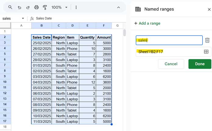
Source File Setup
- Select the data range you want to import (e.g.,
B2:F17). - Click Data > Named Ranges.
- In the Named Ranges panel, enter a name for the range (e.g.,
"Sales"). - Click Done.
- Copy the URL of the source sheet from your browser’s address bar.
Destination File Setup
- Open the destination file where you want to import the data.
- In cell A1, paste the URL of the source sheet.
- In cell A2, enter the name of the named range (
Sales). - In cell A3, enter the formula:
=IMPORTRANGE(A1, A2) - Click Allow Access when prompted.
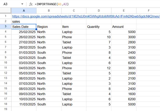
The named range data from the source sheet will now be imported into the destination sheet. Any changes to the named range in the source sheet will automatically reflect in the imported data.
Hardcoding the URL and Named Range
Instead of referencing cells, you can directly enter the IMPORTRANGE formula as:
=IMPORTRANGE("https://docs.google.com/spreadsheets/d/1I62hdJ0mK5WhgXdoMWBfcAd-fFmN2KbwbSgdcNK2mes/edit?gid=0#gid=0", "sales")Additional Tip: Controlling Imported Named Ranges via Drop-Down
If you have multiple named ranges in the source sheet (e.g., Sales, Advance, Purchase_Orders), you can create a drop-down menu to switch between them dynamically.
Steps to Create a Drop-Down for Named Ranges
- In cell A2, click Insert > Drop-down.
- Replace “Option 1” and “Option 2” with the named range names.
- Click Add another item to add more named ranges.
- Once completed, click Done.
Now, selecting a named range from the drop-down will dynamically change the imported data.
FAQs
1. Can I use QUERY with IMPORTRANGE when importing named ranges?
Yes, you can use the QUERY function with IMPORTRANGE as usual. The first column in the named range will be Col1, the second Col2, and so on. Example:
=QUERY(IMPORTRANGE(A1, A2), "select Col1, Col5 Where Col3='Laptop' ", 1)2. What happens if the named range in the source file is broken or deleted?
If the named range is deleted, renamed, or broken in the source file, the IMPORTRANGE function in the destination file will return a #REF! error. This happens because IMPORTRANGE relies on an exact match for the named range.
Solution: Ensure that the named range exists and is correctly referenced in both files. If it was renamed, update the formula in the destination file with the new name.
3. Can I dynamically change the named range being imported?
Yes! You can create a drop-down list containing multiple named ranges and use IMPORTRANGE with a cell reference for dynamic selection.
Resources
- Dynamic Column ID in QUERY IMPORTRANGE Using Named Ranges
- How to Use IMPORTRANGE Function with Conditions in Google Sheets
- Dynamic Sheet Names in IMPORTRANGE in Google Sheets
- How to Use QUERY with IMPORTRANGE in Google Sheets
- Relative Cell Reference in IMPORTRANGE in Google Sheets
- IMPORTRANGE to Import Visible Rows in Google Sheets


My data range isn’t large. Just b2:m9 and I keep getting a
#Referror. Not sure what I am doing wrong. Allowed the permissions and everything.Hi, Stephanie,
Copy the formula and insert it in a new tab. See whether it’s working. If this doesn’t solve the problem, please check what the tooltip (hover your mouse over the error value) says.
How do I allow permissions? It says: “You do not have permission to access that sheet.”
Hi, Melissa,
That means the Sheet belongs to someone else.
Please try the below steps.
1. Copy the URL of the Sheet from the importrange formula.
2. Paste it in the browser address bar and hit enter.
3. Click on “Request access.”
Hi
What’s the limit range to select?
I have thousands of rows and columns till ‘AQ’, After trying the above formula facing the “Result too large” error
Is there any alternate, thanks in Advance.
Hi, Bindu,
Regarding the limitation, Google Sheets Documentation on Importrange says;
So I don’t know exactly the limit of rows and columns in Importrange.
Anyway, you can import the data part by part using multiple Importranges and join them like;
={importrange_output_part_1;importrange_output_part2}Hope this helps?
Best,