The IMPORTRANGE function in Google Sheets does not have an argument that allows you to directly import only the visible rows from one Google Sheets file to another. However, with a workaround, it is possible to import visible rows using IMPORTRANGE.
Before proceeding with the workaround, keep in mind that you need edit access to modify the source file.
Why Do We Require Edit Access?
Edit access is necessary because the workaround involves adding an extra column (a helper column) with a formula in the source file. Without edit access, you cannot modify the source file to include the helper column.
Once the helper column is set up, you can use the QUERY function combined with IMPORTRANGE to import only the visible rows in Google Sheets.
What Are Hidden Rows?
In the context of this tutorial, hidden rows include:
- Rows hidden using the “Hide row” command in the right-click menu.
- Collapsed row groups (using the “Group rows” command in the right-click menu or the View menu).
- Rows filtered out using the “Filter” option in the Data menu.
- Rows filtered out using Slicer
Note: Filtering with a Slicer doesn’t work with the IMPORTRANGE-QUERY combo to import visible rows. This may be a bug requiring developer attention.
How to Import Only Visible Rows Using IMPORTRANGE in Google Sheets
Let’s start with the source file settings. As mentioned earlier, we will be adding a helper column in the source file.
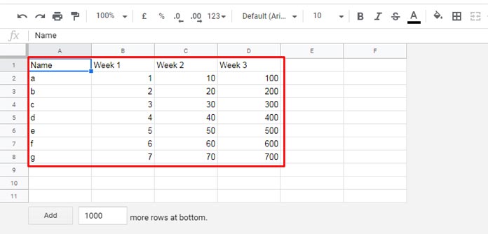
Sample Data to Import (Tab name: ‘kvp1’):
Source File Side – Helper Column Settings
- Make all the rows visible (as shown in my sample data above).
- The last column containing data in my sheet is column D, so we will use column E as the helper column. In cell E1, insert the following formula:
=MAP(A1:A8, LAMBDA(r, SUBTOTAL(103, r)))- Hide the rows you want to (for example, I am hiding rows 3, 4, and 5).
Can You Explain the Formula in Use?
We use SUBTOTAL(103, A1) to return 1 when the row is visible and 0 when it is hidden.
To apply this formula to every row in the range, we convert it into a lambda function as follows:
LAMBDA(r, SUBTOTAL(103, r))We apply this lambda function to each row in the range A1:A8 using the MAP function, which returns an array of 1s for visible rows and 0s for hidden rows.
It will return 1 for visible rows and 0 for hidden rows. Ensure that the range used in the MAP function is not empty to correctly identify the hidden rows.
Destination File Side – QUERY IMPORTRANGE Formula to Import Visible Rows
Imported All Rows:
To import all rows from the source file, follow these steps:
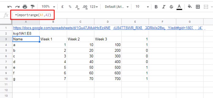
- Copy the URL of the source file from your browser’s address bar and paste it into cell A1 of the destination file.
- In cell A2, enter the range (be sure to include the helper column), such as
kvp1!A1:E8. You can later adjust the rows and columns as needed. - Use the IMPORTRANGE formula in cell A3:
=IMPORTRANGE(A1, A2)You may be prompted to click “Allow Access” to import the data.
Import Visible Rows:
To import only the visible rows, we need to specify a condition. Unfortunately, IMPORTRANGE does not have an argument for conditional imports.
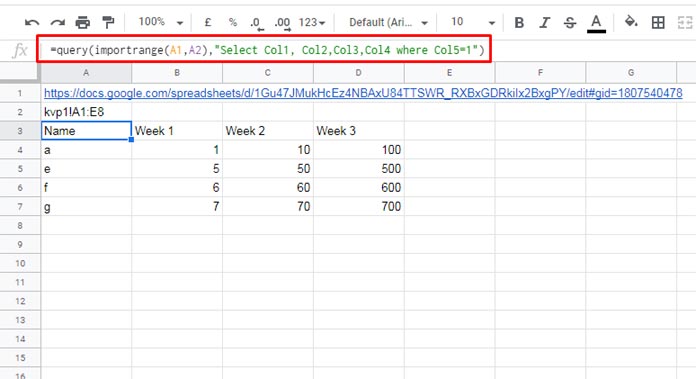
However, we can use the QUERY function with the IMPORTRANGE data to filter the rows based on the helper column. Modify the formula in A3 as follows:
=QUERY(IMPORTRANGE(A1, A2), "SELECT Col1, Col2, Col3, Col4 WHERE Col5 = 1")This will import only the visible rows where the value in column E (the helper column) is 1.


This unfortunately doesn’t work when using Slicers
Thanks for pointing that out! You’re right—Slicers currently don’t work with the IMPORTRANGE-QUERY combo. I’ll update the post to reflect this limitation. Appreciate your feedback!
It’s awesome and so smart!! than others
Great trick. Really informative and useful post.
Thanx and regards