To use a dynamic return column in a VLOOKUP IMPORTRANGE formula in Google Sheets, you must maintain consistent field labels in the source data.
Why Consistent Field Labels Matter
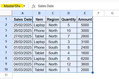
For example, if you want to return the sales amount, use a field label like "Amount" in the corresponding column in the source data. Do not alternate between "Sales Amount" or "Total". Stick to a single label consistently.
In the destination sheet, you can dynamically look up this field label in the header row and determine its column number for use in VLOOKUP.
Aside from this, you can freely add or remove columns in the source data. However, be consistent with the first column, as VLOOKUP searches for the lookup key in this column.
By using a dynamic return column in VLOOKUP IMPORTRANGE, structural changes in the imported data won’t break the formula.
You can move columns around in the range or delete some—except for the first column and the return column label.
Prerequisites for Dynamic Return Column in VLOOKUP IMPORTRANGE
To make this approach work, use a named range in the "range_string" part of IMPORTRANGE instead of a static reference.
IMPORTRANGE Syntax
IMPORTRANGE(spreadsheet_url, range_string)If you use static ranges like "Sheet1!A1:E", changes to the sheet name or data range won’t be reflected in the destination sheet. This increases the risk of formula errors in the future.
Creating a Named Range
To create a named range:
- Select the sample data (e.g., A1:E10).
- Locate the name box (left of the formula bar).
- Click inside it and type a name (e.g.,
"MasterSheet").
How Named Ranges Handle Structural Changes
When you use a named range in IMPORTRANGE, it automatically adapts to changes. Here’s how:
| Action | Effect on Named Range |
| Insert a row or column inside the named range | Named range expands. |
| Delete a row or column inside the named range | Named range shrinks accordingly. |
| Insert or delete a row above the named range | Named range shifts down or up but does not expand. |
| Insert or delete a column before the named range | Named range shifts left or right but does not expand. |
Since named ranges retain these features, they are ideal for importing dynamic data.
Note: Do not move inner columns or rows outside the range. You can rearrange them within the range or move outer columns inside.
Step-by-Step Guide: Dynamic Return Column in VLOOKUP IMPORTRANGE
Follow these steps to create a dynamic return column in VLOOKUP IMPORTRANGE.
Step 1: Import the Named Range
- Copy the URL of the source sheet.
- In cell A1 of the destination sheet, paste the copied URL.
- In cell A2, enter the named range name (
MasterSheet).
Step 2: Define Lookup Values
- In cell A4, enter the field label of the return column (e.g.,
"Amount"). - In cell B4, enter the search key (e.g., a date like
28/02/25). The first column of the imported range contains sales dates, so VLOOKUP will search for this value.
Step 3: Write the VLOOKUP IMPORTRANGE Formula
Use the following formula in cell C4:
=LET(import, IMPORTRANGE(A1, A2), VLOOKUP(B4, import, XMATCH(A4, CHOOSEROWS(import, 1)), FALSE))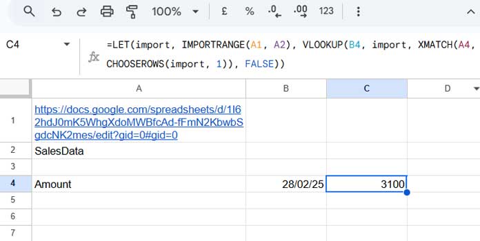
Explanation:
A1-> Contains the source sheet URL.A2-> Contains the named range name (MasterSheet).A4-> Contains the return column label (Amount).B4-> Contains the search key (e.g., a date).IMPORTRANGE(A1, A2)-> Imports data from the named range.XMATCH(A4, CHOOSEROWS(import, 1))-> Finds the column index dynamically based on the header label.VLOOKUP(B4, import, XMATCH(A4, CHOOSEROWS(import, 1)), FALSE)-> Performs the lookup with a dynamic return column.
Why This Works
With this setup, adding or deleting columns won’t require updating the VLOOKUP formula manually. The index column number is determined dynamically using XMATCH and CHOOSEROWS.
Now, VLOOKUP IMPORTRANGE remains robust, even when the imported data changes.
By using a dynamic return column in VLOOKUP IMPORTRANGE, you ensure that your lookup formulas stay functional, even when columns are moved, added, or deleted.


