XLOOKUP with Single IMPORTRANGE & LET in Google Sheets

With the help of the LET function, we can speed up processing when using XLOOKUP with IMPORTRANGE in Google Sheets. This combo allows for the use of a single IMPORTRANGE in an XLOOKUP operation.

However, if you’d rather skip LET and go for a single IMPORTRANGE, you’ll need a helper range to store the imported data.

Some might wonder, why not just use VLOOKUP with IMPORTRANGE to fix this?

Indeed, VLOOKUP needs a range, so you won’t need multiple IMPORTRANGE for the lookup. However, the problem is that it looks for the key only in the first column of the range.

To address this, you can use CHOOSECOLS. However, VLOOKUP lacks several XLOOKUP features, such as searching from the last value to the first value and specifying a ‘missing value,’ among others.

Now, let’s delve into how to use XLOOKUP with a single IMPORTRANGE without resorting to helper columns or ranges in Google Sheets.

XLOOKUP with Single IMPORTRANGE for Vertical Lookup

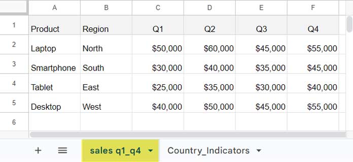
We have a Google Sheets table in the range A:F, illustrating sales data for various products across different regions.

Within this table, the field labels in A1:F1 are as follows: Product, Region, Q1, Q2, Q3, and Q4. The corresponding columns contain the following relevant data:

“Product” in Column A signifies the type of product being sold.
“Region” in Column B denotes the geographic area of sales.
Columns C to F house the sales data for each “Q1,” “Q2,” “Q3,” and “Q4” respectively.

Refer to the screenshot below and take note of the tab name, which is ‘sales q1_q4,’ because when importing data into another Google Sheets file, we will use the sheet name with the range, such as ‘sales q1_q4!A:F.’

Sample Sales Data: Contains Product, Region, Q1-Q4 Data

Prerequisites

Before utilizing the XLOOKUP with a single IMPORTRANGE formula to enhance performance, we must ensure that the IMPORTRANGE correctly imports data. So initially, we will import the data and then delete it. Here are the steps:

Copy the URL of the sample sheet containing the sales data from the browser’s address bar.
In a new Google Sheets file, enter the following formula in cell A1:

=IMPORTRANGE("spreadsheet_url", "sales q1_q4!A:F")

Replace spreadsheet_url with the copied URL. After entering the formula, it may return a #REF! error. Hover over this error, and you will see an option to “Allow Access.” Clicking on it will import the data.

In the next step, we will incorporate this formula within LET, assign it a name, and then use that name in XLOOKUP. Let’s proceed with these steps in the examples below.

Single Search Key and Single Output (Single Column Result Range)

Instead of providing the formula outright, let’s break down the code step by step to enhance your proficiency in using XLOOKUP with IMPORTRANGE.

Assume you want to find the product “Smartphone” in column A and retrieve the Q4 sales quantity from column F. Typically, we use the following XLOOKUP formula.

=XLOOKUP("Smartphone", A:A, F:F)

We can rewrite the formula as follows to use a range instead of specific columns.

=XLOOKUP("Smartphone", CHOOSECOLS(A:F, 1), CHOOSECOLS(A:F, 6))

The CHOOSECOLS function retrieves the first column (A:A) in the lookup range and the sixth column (F:F) in the result range.

Instead of using the range A:F twice in the formula (as seen in the two CHOOSECOLS), we can assign it a name like “data” and use that name instead. For this, we need to use the LET function. Here is that formula:

=LET(data, A:F, XLOOKUP("Smartphone", CHOOSECOLS(data, 1), CHOOSECOLS(data, 6))

Now, for XLOOKUP with a single IMPORTRANGE, replace A:F with the IMPORTRANGE formula itself.

=LET(data, IMPORTRANGE("spreadsheet_url", "sales q1_q4!A:F"), XLOOKUP("Smartphone", CHOOSECOLS(data, 1), CHOOSECOLS(data, 6)))

Enter the search_key “Smartphone” in cell A1 and use the above formula with the following correction in cell B1:

=LET(data, IMPORTRANGE("spreadsheet_url", "sales q1_q4!A:F"), XLOOKUP(A1, CHOOSECOLS(data, 1), CHOOSECOLS(data, 6)))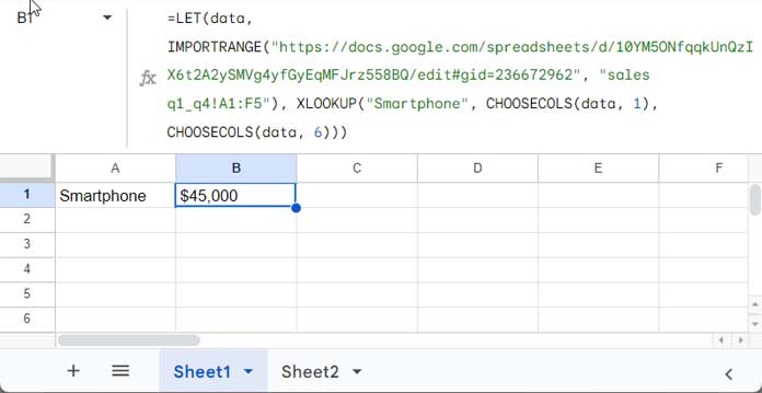

Single Search Key and Multiple Column Output (Multiple Column Result Range)

How do we check the sales amount of the “Smartphone” in Q1, Q2, Q3, and Q4?

In the above formula, the lookup range is A:A, i.e., CHOOSECOLS(data, 1). You don’t need to make any changes to it. However, you should make changes to the result range, i.e., CHOOSECOLS(data, 6).

It should be C:F, and you can refer to that using CHOOSECOLS(data, {3, 4, 5, 6}).

So, the XLOOKUP with a single IMPORTRANGE formula will become:

=LET(data, IMPORTRANGE("spreadsheet_url", "sales q1_q4!A:F"), XLOOKUP(A1, CHOOSECOLS(data, 1), CHOOSECOLS(data, {3, 4, 5, 6})))

The formula will return the Q1, Q2, Q3, and Q4 sales amount of “Smartphone,” which is $30,000, $40,000, $35,000, and $45,000, respectively.

XLOOKUP with IMPORTRANGE: Vertical Lookup Using Multiple Search Keys

Single Column Result Range:

Assume you want the Q4 sales price of the products Smartphone and Tablet, which are in cells A1 and A2, respectively.

You can specify the range A1:A2 in XLOOKUP and enter the formula as an array formula:

=ArrayFormula(LET(data, IMPORTRANGE("spreadsheet_url", "sales q1_q4!A:F"), XLOOKUP(A1:A2, CHOOSECOLS(data, 1), CHOOSECOLS(data, 6))))

Multiple Column Result Range:

What about extracting the Q1, Q2, Q3, and Q4 sales amount of both “Smartphone” and “Tablet” in A1:A2?

Replacing CHOOSECOLS(data, 6) with CHOOSECOLS(data, {3, 4, 5, 6}) won’t help here. You need an additional step.

First, replace CHOOSECOLS(data, 6) with CHOOSECOLS(data, {3, 4, 5, 6}) in the above formula. Then remove the ArrayFormula function:

LET(data, IMPORTRANGE("spreadsheet_url", "sales q1_q4!A:F"), XLOOKUP(A1:A2, CHOOSECOLS(data, 1), CHOOSECOLS(data, {3, 4, 5, 6})))

Keep it aside.

We can use the MAP function to iterate over the search keys and obtain a 2D result from the XLOOKUP with a single IMPORTRANGE formula.

The search key range is A1:A2. In MAP, you should specify it as the array argument, like =MAP(A1:A2, LAMBDA(val,

where val represents the current element in the array A1:A2.

Now, copy the above formula, which we kept aside, and paste it within the lambda to act as the function. Don’t forget to replace A1:A2 within the XLOOKUP with val.

=MAP(A1:A2, LAMBDA(val, LET(data, IMPORTRANGE("spreadsheet-url", "sales q1_q4!A:F"), XLOOKUP(val, CHOOSECOLS(data, 1), CHOOSECOLS(data, {3, 4, 5, 6})))))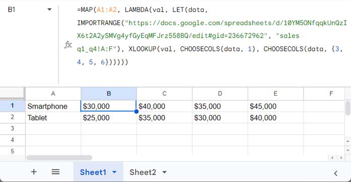

XLOOKUP with Single IMPORTRANGE for Horizontal Lookup

Horizontal lookup is less common, as most of us typically work with vertical data. Since the above formula requires minor modifications to perform a horizontal lookup, let me explain that too.

This time, the sample data is in 1:5, where A1:A5 contains the field labels: Country, Population, GDP, HDI, and Area (sq km). The relevant data is spread across each corresponding row.

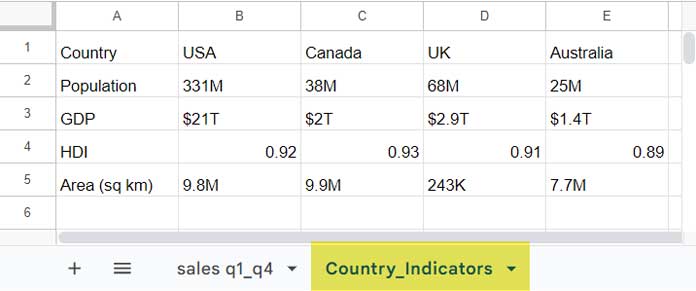
Sample Country Indicators Data: Contains Country, Population, GDP, HDI, Area

The sheet name is ‘Country_Indicators.’ So, you can import it as before using the following formula:

=IMPORTRANGE("spreadsheet_url", "Country_Indicators!1:5")

Replace spreadsheet_url with the URL of the file that contains the above data.

Single Search Key and Single Output (Single Row Result Range)

To search for the country “UK” in the first row and return the value from the corresponding column in the fifth row, we can use the following formula:

=XLOOKUP("UK", 1:1, 5:5)

We can replace the lookup range and result range with CHOOSEROWS as follows:

=XLOOKUP("UK", CHOOSEROWS(1:5, 1), CHOOSEROWS(1:5, 5))

The CHOOSERPWS function retrieves the first row (1:1) in the lookup range and the fifth row (5:5) in the result range.

Let’s use LET to name the range 1:5 as “data” and replace 1:5 in CHOOSEROWS with that name.

=LET(data, 1:5, XLOOKUP("UK", CHOOSEROWS(data, 1), CHOOSEROWS(data, 5))

Now, we are set to incorporate IMPORTRANGE within this combination of LET, CHOOSEROWS, and XLOOKUP. For that, replace the range 1:5 with the IMPORTRANGE formula itself.

=LET(data, IMPORTRANGE("spreadsheet_url", "Country_Indicators!1:5"), XLOOKUP("UK", CHOOSEROWS(data, 1), CHOOSEROWS(data, 5)))

Specify the criterion “UK” in cell A1 and replace “UK” in the formula with the reference to cell A1:

=LET(data, IMPORTRANGE("spreadsheet_url", "Country_Indicators!1:5"), XLOOKUP(A1, CHOOSEROWS(data, 1), CHOOSEROWS(data, 5)))

Single Search Key and Multiple Row Output (Multiple Row Result Range)

If you want to horizontally look up the country name in the first row and return Population, GDP, HDI, and Area (sq km) from rows 2 to 5, make the following changes in the above XLOOKUP with IMPORTRANGE formula:

The result range in the above formula is CHOOSEROWS(data, 5). You should replace that with CHOOSEROWS(data, {2, 3, 4, 5})

=LET(data, IMPORTRANGE("spreasheet_url", "Country_Indicators!1:5"), XLOOKUP(A1, CHOOSEROWS(data, 1), CHOOSEROWS(data, {2, 3, 4, 5})))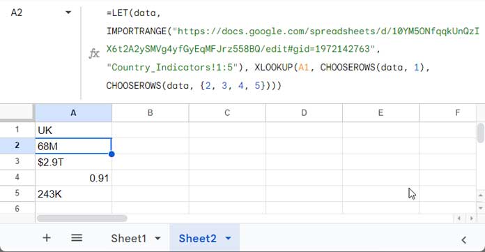

XLOOKUP with a Single IMPORTRANGE for Horizontal Lookup

XLOOKUP with IMPORTRANGE: Horizontal Lookup Using Multiple Search Keys

This is similar to a vertical lookup, where we have specified multiple criteria in a column range, i.e., in A1:A2. But this time, we should specify them in a row range, for example, in A1:B1.

Enter “UK” in cell A1 and “Australia” in cell B1. If your result range contains a single row, use A1:B1 as the search key and enter the formula as an array formula.

Example:

=ArrayFormula(LET(data, IMPORTRANGE("spreadsheet_url"), XLOOKUP(A1:B1, CHOOSEROWS(data, 1), CHOOSEROWS(data, 5))))

If the result range contains multiple rows, then you must use the MAP function as follows.

Specify the array A1:B1 in MAP and name it “val.” That part of the MAP will be as follows: =MAP(A1:B1, LAMBDA(val,

The function in the Lambda is the XLOOKUP with the IMPORTRANGE formula above. You need to replace A1:B1 in that formula with val, remove ArrayFormula, and replace CHOOSEROWS(data, 5) with CHOOSEROWS(data, {2, 3, 4, 5}). Here it is:

=MAP(A1:B1, LAMBDA(val, LET(data, IMPORTRANGE("spreadsheet_url", "Country_Indicators!1:5"), XLOOKUP(val, CHOOSEROWS(data, 1), CHOOSEROWS(data, {2, 3, 4, 5})))))

Resources

We have seen examples of how to use XLOOKUP with IMPORTRANGE in both vertical and horizontal datasets. Here are some other XLOOKUP tips and tricks: