Say goodbye to repetitive formatting! This guide shows you how to create Google Sheets tables that automatically mimic the style of the last row, saving you precious time and effort.
This becomes especially handy if you utilize cell formatting like fill color, bold, italics, font size, underline, and features such as drop-downs and checkboxes.
As your table expands, Google Sheets will preserve the formatting from the last row entry. If there are drop-downs or checkboxes, they will seamlessly extend to the new row.
However, it’s essential to note that formulas won’t automatically inherit unless you’re employing array formulas.
While not a novel concept, Google Sheets inherently includes this feature, although it differs from Excel’s “Format as Table.”
Let’s explore how to set up a self-formatting table as it grows. We will create a table in Google Sheets and demonstrate how to apply formatting that remains inherent as the table grows.
Creating a Basic Table with Sample Data
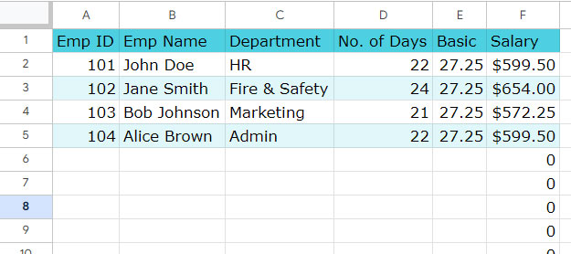
Here is some sample employee data that you can copy into a blank Google Sheets file in the cell range A1:F5:
| Emp_ID | Name | Department | No. of Days | Basic (Per Day) | Salary |
| 101 | John Doe | HR | 22 | 27.25 | |
| 102 | Jane Smith | Fire & Safety | 24 | 27.25 | |
| 103 | Bob Johnson | Marketing | 21 | 27.25 | |
| 104 | Alice Brown | Admin | 22 | 27.25 |
This type of tabular data is useful for sorting, filtering, creating Pivot Tables, and applying formulas for various data manipulations.
This is the basic step of creating a table that inherits the last row’s format (in this case, A5:F5) when you add rows (records) below. Let’s first apply some basic formatting to this table manually.
Inserting Necessary Array Formulas
Replace the existing field label in cell F1 with the following array formula to calculate the salary based on the number of days present.
=ArrayFormula(IF(ROW(D:D)=1,"Salary", D:D*E:E))This formula is designed to expand dynamically with the table.
If you anticipate the table growing in the future, using array formulas in the top row of the table, as shown above, ensures that the formula result expands accordingly.
Formatting the Table
Without incorporating basic formatting to the created table, such as currency formatting, bold values, and applying drop-downs and filters, we won’t be able to test how the table inherits formatting as it grows. Here are some essential formatting and other settings.
Applying Currency Formatting:
- Select F2:F5.
- Click Format > Number > Custom Currency.
- Choose “US Dollar” and click Apply.
Applying Alternating Colors:
- Select the table range A1:F5.
- Click on Format > Alternating Colors.
This will apply alternating colors to the table, expanding as the table grows. Choose styles from the sidebar panel.
Related: Applying Alternating Colors to Visible Rows in Google Sheets & Excel.
Applying Filter to the Table:
- Select A1:F5.
- Click on Data > Create a filter. This adds a filter to the table.
Creating a (Data Validation) Drop-Down:
- Select C2:C5.
- Click Insert > Drop-Down.
Google Sheets will use all the values in C2:C5 to insert drop-downs in the selected range. It overwrites the existing values with drop-downs, but the active value will be the one present before inserting the drop-down.
You May Like: The Best Data Validation Examples in Google Sheets.
Bold the Name in Cell B5:
Bold the name in cell B5 and increase the font size.
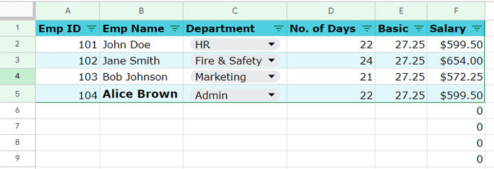
The above formatting will help you understand whether Google Sheets maintains the formatting of the last row or the entire table as it grows.
The Crucial Step in Creating Self-Formatting Tables in Google Sheets
Here is the crucial step in creating a self-formatting table in Google Sheets.
You need to delete all the rows after the last records in the table, meaning you should delete all rows from row #6 to the last row in the sheet.
This final step is essential to create a self-formatting table. Here are the steps to follow:
- Click on the row number 6 (the first row you want to delete).
- Hold down the Shift key and press the down arrow key until you reach the very last row of your spreadsheet. This will select all rows from 6 to the end.
- Right-click anywhere within the selected rows.
- Choose “Delete selected rows” from the context menu.
We are now ready to test the table feature in Google Sheets!
Adding New Records to the Table
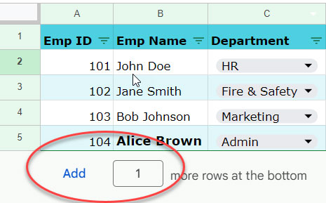
To inherit the formatting from the last row of the created table, add one row each time you input a record.
Type ‘1’ in the field next to ‘Add’ and click the ‘Add’ button. This process can be simplified using a keyboard shortcut in both Windows and Mac.
Navigate to any cell in the last row (in this example, row 5) and press Alt + I + R + B on Windows or Alt + Shift + I + R + B on Mac to insert a new row at the bottom. This shortcut is easy to remember as the keys ‘I,’ ‘R,’ and ‘B’ correspond to ‘Insert Row Bottom.
Add one row at the bottom and enter some values in the added row. You’ll observe that our table inherits the formatting, including drop-downs, from the immediate row above.
Key Takeaways: Creating Self-Formatting Tables in Google Sheets
Here are the key takeaways from the above tutorial:
- To create a dynamic table that expands with formatting, follow these steps: enter your data, apply the desired formatting, and delete all other rows. Google Sheets automatically extends formatting to new rows, saving you time and effort.
- Unlike Excel, Google Sheets allows you to keep the required rows and add new ones as needed. It’s recommended to add one row at a time, though this may seem tedious. To streamline the process, make use of keyboard shortcuts.
- By following this approach, you can ensure that the last row’s formatting is retained for newly added records.
This allows you to create a proper table in Google Sheets.


