Control Reloading of Importrange from the Source File in Google Sheets

Here is a workaround to control reloading of the Importrange data in the destination file from the source file in Google Sheets. Honestly, I’m unsure whether this method is fully effective or not. Please test it yourself to know.

Here is the scenario where this kind of controlling of importing of cells or range of cells from one Spreadsheet to another comes useful.

Assume, I have given Importrange access to one of my Google Sheets to my employees. So that they can import certain data from my sheet to their sheets.

I’ll update my sheet often. But I want to have some type of control over the updated data. Didn’t get?

Understand Controlling Reloading of Importrange Data

Assume the data I am sharing with my employees is a job schedule.

I may update the schedule frequently based on the progress of the job. Some times to incorporate the progress or sometimes to re-arrange the schedule to focus on the backlogs.

I don’t want them (my employees) to see what I am doing in the background. The employees should only see the old schedule until I push the new data to them.

That means I want some type of control like a tickbox to control reloading of Importrange data in their sheet from my source file.

In concise, I want Importrange in their files to keep the old data while I am editing the source. Still, having any doubt? The example below will hopefully help you understand it.

Workaround to Control Reloading of Importrange Data from the Source Sheet

In this example, I am just importing a four-column data from one Google Sheets file to another with the help of the Importrange function.

Considering the ease of understanding, let’s call the files by the names ‘Source File’ and ‘Destination File’. We require one more file as a ‘bridge’ from ‘Source File’ to ‘Destination File’. I’ll give the name of that sheet later.

The ‘Source File’ has four tabs – ‘Sch’, ‘New’, ‘Old’, and ‘Control’.

Below you can find the purpose of each tab in a nutshell. The detailed explanation follows after that under different subtitles.

The last 3 tabs have been created as per my workaround to control reloading of Importrange in the ‘Destination File’ from within the ‘Source File’.

The ‘New’ tab copies data from the ‘Sch’ tab (which is the master sheet containing my schedule) based on enabling a tick box in the ‘Sch’ tab. It’ll always have the same data from the ‘Sch’ tab unless I uncheck the tick box.

The ‘Old’ tab contains the backup of the ‘Sch’ tab which copied manually. Before updating the ‘Sch’ tab, always copy-paste all the values from it, except the tick box, to the ‘Old’ tab.

Using the ‘Control’ tab we can control reloading of the Importrange from the source, i.e. from the ‘Control’ tab in the ‘Source File’, in Google Sheets. I mean we can decide which data to serve to the ‘Destination File’.

Source File – Sch, New, Old, and Control Tabs and Their Purpose in Importrange

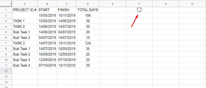
Data in the ‘Sch’ Sheet

This tab contains the source data to import to the ‘Destination File’. I’may update this tab frequently.

Tick Box to Enable or Disable Importing of Data in Sheets

Please take a note of the tick box in cell F1 in this tab. I’ll explain the purpose of it later. To insert a tick box, go to the Insert menu. There you can find the Tick box option.

Must Read: 10 Best Tick Box Tips and Tricks in Google Sheets.

Data in the ‘New’ Sheet

In cell A1 in this tab, I have the following formula which pulls the data from the ‘Sch’ tab, conditionally.

=if(Sch!F1=TRUE,ArrayFormula(Sch!A1:D),"Please check back later")

If the tick box is enabled (checked) in cell F1 in the ‘Sch’ tab, the data in the range A1:D will be copied to this tab (‘New’ tab). Else, if unchecked, the formula will show a custom message saying “Please check back later”.

Data in the ‘Old’ Sheet

The exact copy or backup of the ‘Sch’ tab. So I am not posting the screenshot again.

Data in the ‘Control’ Sheet to Control the Reloading of Importrange from the Source File

Using this sheet we can control which data new/old to push to the employees (Destination File).

Control Reloading of Importrange Data in Google Sheets

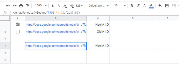
In cell A1 and A2, you can see two tick boxes. To insert multiple tick boxes, simply select the range (here cell A1 and A2) and go to the Insert menu and click on the Tick box.

The cell B1 and B2 contain the URLs of the tab ‘New’ and ‘Old’ respectively. To get the URL, go to each tab and copy the URLs from the address bar of the browser. Their corresponding range to export has been specified in cell C1 and C2.

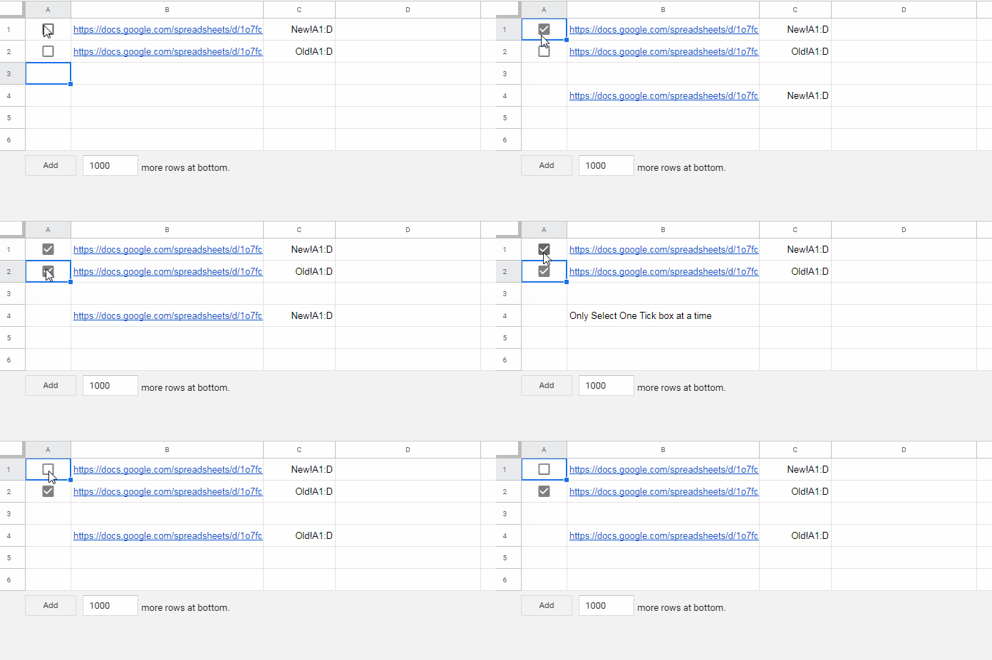
If you enable, I mean click on the first tick box, the destination file will have the data from the ‘New’ tab. If you enable the second tick box, then the destination file will retain the ‘Old’ tab data.

How? The answer is the Vlookup in cell B4 in the ‘Control’ tab.

=if(countif(A1:A2,true)=2,"Only Select One Tick box at a time",ArrayFormula(IFNA(vlookup(TRUE,A1:C2,{2,3},0))))

In B4:C4, it populates the URL and range to be used in the Importrange in the ‘Destination File’. The tick box controls the URL and the range.

Changes in File Sharing Settings (Source File)

Now go to the File menu and click on ‘Share’ and change the sharing settings to ‘Private – Only you can access’ also called ‘OFF- Specific people’. Copy the Link.

Mirror File (Bridge) to Control Reloading of Importrange

I have mentioned about a third file, which acts as a ‘bridge’, in the beginning, right? I was talking about this file named ‘Mirror File’.

As part of controlling the reloading of Importrange in Google Sheets, in this file, we require only one tab. Name it as ‘Mirror’. In the very first cell, enter the below formula.

=importrange(importrange("Source File URL Here","'Control'!B4"),importrange("Source File URL Here","'Control'!C4"))

Please don’t forget to replace the Source File URL Here in the formula with the URL of the ‘Source File’ which you have copied at the time of changing the File sharing setting above.

Changes in File Sharing Settings (Mirror File)

File > Share > Advanced > On – Anyone with the link (Anyone who has the link can view). Copy the Link.

Destination File – Importrange Formula that Responds to User Action in the Source

Here is the final step to control reloading of Importrange in the ‘Destination File’ from the ‘Source File’ in Google Sheets.

In cell A1 in the ‘Destination File’, enter the following formula.

=importrange("Mirror File URL Here","Mirror!A1:D")

Replace Mirror File URL Here with the copied link.

How does the above controlling, reloading of the Importrange in Google Sheets works?

See the below table.

IMPORTRANGE CONTROLS (SOURCE FILE)	IMPACT ON THE RELOADING (DESTINATION FILE)
When Tick box enabled in ‘Sch’ F1
‘Control’ tab A1 checked, A2 Unchecked	Imports all the data from the ‘New’ tab to the ‘Destination File’.
‘Control’ tab A2 checked, A1 Unchecked	Imports all the data from the ‘Old’ tab to the ‘Destination File’.
When both the tick boxes enabled or disabled	#N/A!
When Tick box disabled in ‘Sch’ F1
Control tab A1 checked, A2 Unchecked	Shows a custom message saying “Please check back later”.

That’s all about control reloading of Importrange in Google Sheets. Enjoy!

How to Control Reloading of Importrange from the Source File in Google Sheets