How to Use IMPORTRANGE with FILTER in Google Sheets

You can use IMPORTRANGE with FILTER in Google Sheets to import only the rows that match specific conditions from another spreadsheet. This approach is especially useful when the source data contains mixed data types that the QUERY function may not handle correctly.

Before the LET function was introduced, using IMPORTRANGE with FILTER often required either a helper imported range or repeating the IMPORTRANGE formula for both the imported range and the filter conditions. Since IMPORTRANGE retrieves data from another spreadsheet, repeating it can slow down recalculation.

With LET, you can store the imported data in a variable and reuse it within FILTER, avoiding repeated IMPORTRANGE calls and improving performance.

The easiest way to build the formula is step by step. First, make sure IMPORTRANGE works correctly. Then wrap it with LET and FILTER.

Quick Answer: Use LET to store the IMPORTRANGE result and pass it to FILTER. This avoids repeating IMPORTRANGE, improves performance, and makes the formula easier to read.

=LET(
  import, IMPORTRANGE(spreadsheet_url, range_string),
  FILTER(import, condition1, [condition2, ...])
)

Table of Contents

Step 1: Import the Data

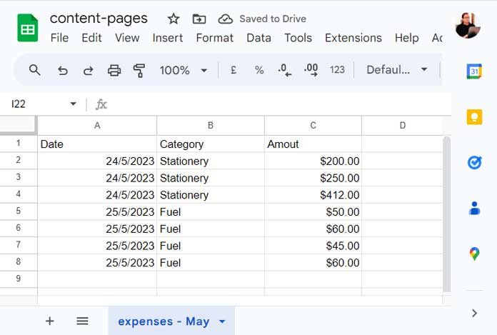
Assume you want to import data from the expenses – May sheet in the content-pages spreadsheet.

Source data in the expenses - May sheet for the IMPORTRANGE example

The syntax is:

=IMPORTRANGE(spreadsheet_url, range_string)

Replace:

spreadsheet_url with the URL of the source spreadsheet.
range_string with the range to import, for example:'expenses - May'!A1:C

After entering the formula for the first time, Google Sheets displays a #REF! error asking for permission to connect the two spreadsheets.

Click Allow access, and the imported data will appear.

Step 2: Use IMPORTRANGE with FILTER

Once you’ve confirmed that IMPORTRANGE works correctly, wrap it with LET and FILTER.

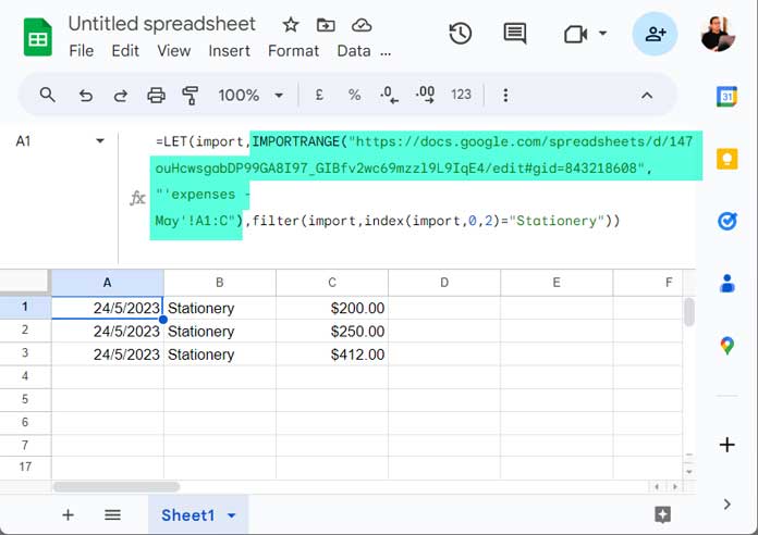
Suppose you want to import only the rows where the Category (the second column) is “stationery”.

=LET(
  import,
  IMPORTRANGE(
    "source_spreadsheet_url",
    "expenses - May!A1:C10"
  ),
  FILTER(
    import,
    INDEX(import, 0, 2)="stationery"
  )
)

Note: Replace source_spreadsheet_url with the URL of your source spreadsheet.

IMPORTRANGE with FILTER formula using LET to import rows matching one criterion

In this formula:

LET stores the imported data in the variable import.
FILTER returns only the matching rows.
INDEX(import, 0, 2) returns the second column from the imported range.
The 0 tells INDEX to return all rows.
Instead of INDEX(import, 0, 2), you can also use CHOOSECOLS(import, 2).

Because the imported data is stored only once, Google Sheets doesn’t need to evaluate IMPORTRANGE multiple times.

Multiple Criteria in IMPORTRANGE with FILTER

To apply multiple conditions, simply add more conditions to FILTER.

For example, to import only rows where:

Category = stationery
Amount > 100

use:

=LET(
  import,
  IMPORTRANGE(
    "source_spreadsheet_url",
    "expenses - May!A1:C"
  ),
  FILTER(
    import,
    INDEX(import, 0, 2)="stationery",
    INDEX(import, 0, 3)>100
  )
)

Using Cell References as Criteria

Instead of hardcoding the criterion, you can reference a cell.

For example, if E1 contains the category to filter:

=LET(
  import,
  IMPORTRANGE(
    "source_spreadsheet_url",
    "expenses - May!A1:C"
  ),
  FILTER(
    import,
    INDEX(import, 0, 2)=E1
  )
)

Changing the value in E1 automatically updates the imported results.

Why Use LET with IMPORTRANGE?

Without LET, the common approach was similar to:

=FILTER(
  IMPORTRANGE(...),
  INDEX(IMPORTRANGE(...), 0, 2)="stationery"
)

Notice that IMPORTRANGE appears twice.

Since IMPORTRANGE retrieves data from another spreadsheet, each occurrence may trigger another import operation. As your spreadsheet grows or the number of conditions increases, recalculation can become noticeably slower.

Using LET imports the data only once and reuses it throughout the formula, making it easier to read and more efficient.

QUERY or FILTER with IMPORTRANGE?

Both QUERY and FILTER work well with IMPORTRANGE. The better choice depends on your data and the task.

Use QUERY	Use FILTER
Filtering and aggregation	Simple row filtering
SQL-like query syntax	Easier to learn
Structured datasets	Mixed data types
Sorting and grouping in one formula	Straightforward logical conditions

In general:

Use QUERY when you need filtering, sorting, grouping, or aggregation in a single formula.
Use FILTER when you only need to return matching rows or when the source data contains mixed data types that QUERY may not interpret correctly.