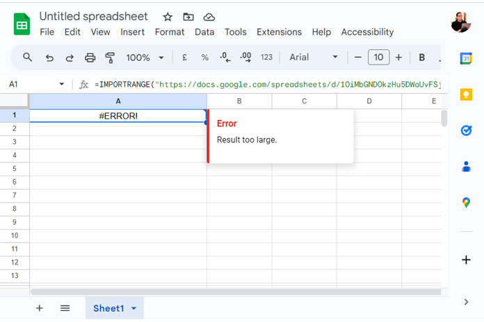
HomeGoogle DocsSpreadsheetIMPORTRANGE Result Too Large Error: Solution

IMPORTRANGE Result Too Large Error: Solution

Published on

If you are importing large volumes of data, you may eventually encounter the IMPORTRANGE “Result too large” error.

We can use the VSTACK or HSTACK functions to work around the “Result too large” error in Google Sheets.

The IMPORTRANGE function returns the #ERROR! value, when the number of cells to import is above its capability.

A quick solution to this problem is to import the data part by part and stack them. You can also use the QUERY function together with each imported data before stacking to enhance the performance.

The number of cells that can be imported using the IMPORTRANGE function is limited. This limit may vary from user to user depending on the types of data in the cells.

Since there is no official documentation on the exact limit, it is difficult to say exactly how many cells can be imported.

I recently got the “Result too large” error when I tried to import 26 columns and 20,000 rows. If I specified 12,606 rows with that many columns, the formula worked flawlessly. However, for my particular data, it could not handle more than that.

I solved this problem in two ways. In the first approach, I imported every 10,000 rows and 26 columns and stacked them vertically.

In the second approach, I imported 20,000 rows and 13 columns each and stacked them horizontally.

Below in the next section, we will see how to use the VSTACK and HSTACK functions with multiple IMPORTRANGE formulas to solve the “Result too large” error.

VSTACK with IMPORTRANGE and the Result Too Large Error

Formula Example:

=LET(url,"https://docs.google.com/spreadsheets/d/1OiMbGNDOkzHu5DWaUvFSj_5cdq3rhvqu-ocWeXhbflo/edit#gid=1707494620",VSTACK(IMPORTRANGE(url,"Sheet2!A1:Z10000"),IMPORTRANGE(url,"Sheet2!A10001:Z20000")))

Syntax: IMPORTRANGE(spreadsheet_url, range_string)

The role of LET in this formula is to assign the “spreadsheet_url” to the name url. This allows us to avoid repeating it in IMPORTRANGES.

In short, we have assigned the “spreadsheet_url” to the name url outside the IMPORTRANGE function. Therefore, within the function, we can use the name url instead. This dramatically reduces the length of the formula.

There are two IMPORTRANGE formulas nested within the VSTACK function.

  1. IMPORTRANGE(url,"Sheet2!A1:Z10000")
  2. IMPORTRANGE(url,"Sheet2!A10001:Z20000")

You can add more IMPORTRANGE formulas after the second one, separated by a comma.

Let’s now move on to the HSTACK solution to the #ERROR! Result too large errors.

HSTACK with IMPORTRANGE and the Result Too Large Error

Formula Example:

=LET(url,"https://docs.google.com/spreadsheets/d/1OiMbGNDOkzHu5DWaUvFSj_5cdq3rhvqu-ocWeXhbflo/edit#gid=1707494620",HSTACK(IMPORTRANGE(url,"Sheet2!A1:M20000"),IMPORTRANGE(url,"Sheet2!N1:Z20000")))

There are two IMPORTRANGE formulas nested within the HSTACK function. The first formula returns the first 13 columns, and the second formula returns the next 13 columns.

  1. IMPORTRANGE(url,"Sheet2!A1:M20000")
  2. IMPORTRANGE(url,"Sheet2!N1:Z20000")

Here also, you can add more IMPORTRANGE formulas after the second one, separated by a comma.

How can I improve the performance of importing large volumes of data?

We now have two solutions to solve the IMPORTRANGE Result too large error. These are the VSTACK + IMPORTRANGE and HSTACK + IMPORTRANGE methods.

However, there are certain things that you can consider to improve their performance.

One option is to use the QUERY function with them to filter rows of IMPORTRANGE imported data, thereby cutting short its length.

When you use the QUERY function with VSTACK + IMPORTRANGE, you can use it to filter rows conditionally. This can shrink the data. For example, you can use the following formula to filter out blank rows based on column 5:

=LET(url,"https://docs.google.com/spreadsheets/d/1OiMbGNDOkzHu5DWaUvFSj_5cdq3rhvqu-ocWeXhbflo/edit#gid=1707494620",VSTACK(QUERY(IMPORTRANGE(url,"Sheet2!A1:Z10000"),"Select * where Col5 is not null"),QUERY(IMPORTRANGE(url,"Sheet2!A10001:Z20000"),"Select * where Col5 is not null")))

What about using the QUERY function with HSTACK and IMPORTRANGE? You can use this combination to remove columns.

Here is an example formula:

=LET(url,"https://docs.google.com/spreadsheets/d/1OiMbGNDOkzHu5DWaUvFSj_5cdq3rhvqu-ocWeXhbflo/edit#gid=1707494620",HSTACK(QUERY(IMPORTRANGE(url,"Sheet2!A1:M20000"),"Select Col1,Col2,Col3"),QUERY(IMPORTRANGE(url,"Sheet2!N1:Z20000"),"Select Col10,Col11,Col12")))

Remember one thing: each formula returns 13 columns. So, in QUERY, you can select columns from 1 to 13 in each formula, not 1-13 in the first formula and 14-26 in the second formula.

If you want to learn more about filtering IMPORTRANGE, please check out my following tutorials.

  1. IMPORTRANGE Within FILTER Function in Google Sheets.
  2. How to Use IMPORTRANGE Function with Conditions in Google Sheets.
  3. How to Use Query with Importrange in Google Sheets.

Conclusion

In short, these are the methods to solve the IMPORTRANGE “Result too large” errors and enhance performance:

  1. Split the data into smaller chunks and import each chunk. Join the data then using the VSTACK or HSTACK function. This can reduce the amount of data that is imported at once.
  2. Use QUERY to filter rows conditionally. This can shrink the data.
  3. Use QUERY to remove columns. This can reduce the number of columns.
Prashanth KV
Prashanth KV
Your Trusted Google Sheets and Excel Guide Prashanth KV brings a wealth of experience in Google Sheets and Excel, cultivated through years of work with multinational corporations in Mumbai and Dubai. As a recognized Google Product Expert in Docs Editors, Prashanth shares his expertise through insightful blogging since 2012. Explore his blog for practical tips and guidance on maximizing your spreadsheet skills.

Get the First or Last Row/Column in a New Google Sheets Table

If you've recently started using the new Google Sheets TABLE functionality, you may find...

UNIQUE Function in Visible Rows in Google Sheets

The UNIQUE function doesn't inherently include only visible rows when it returns values, discarding...

Customizing Alternating Colors of a Table in Google Sheets

Google Sheets' new table feature offers limited options for customizing colors. While you can...

Structured Table References in Formulas in Google Sheets

When you create a Google Sheets table by inserting custom tables or converting a...

More like this

Get the First or Last Row/Column in a New Google Sheets Table

If you've recently started using the new Google Sheets TABLE functionality, you may find...

UNIQUE Function in Visible Rows in Google Sheets

The UNIQUE function doesn't inherently include only visible rows when it returns values, discarding...

Customizing Alternating Colors of a Table in Google Sheets

Google Sheets' new table feature offers limited options for customizing colors. While you can...

LEAVE A REPLY

Please enter your comment!
Please enter your name here

This site uses Akismet to reduce spam. Learn how your comment data is processed.