In Google Sheets, adding blank rows between each group in your data can be quite tedious if done manually.
We can streamline this process by using a formula to automatically insert ‘n’ blank rows between each group in Google Sheets. This approach leverages modern Google Sheets functions.
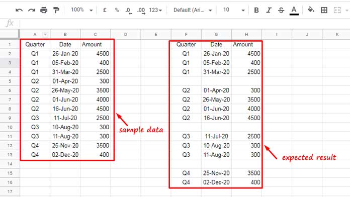
Refer to the illustration below for sample data in range A1:C and the expected output in range F1:H.
We can use either lambda or non-lambda formulas to solve this. We will explore both options. It’s important to note that lambda functions may impact Sheets’ performance.
Formula to Insert Blank Rows Between Each Group: Non-Lambda Approach
Based on the example provided (see Figure 1 above), the group column is column A (Quarter).
I aim to separate each “Quarter” by inserting a blank row after each group. For example, inserting a blank row after each group Q1, Q2, Q3, and Q4.
According to the sample data in range A1:C, the blank rows should be inserted after row #4, row #8, and row #11, which means after the end of each category.
Formula:
=ArrayFormula(
   LET(
      lr, XMATCH(TRUE, A:A<>"", ,-1),
      data, INDIRECT("A2:C"&lr),
      gc, INDIRECT("A2:A"&lr),
      ugc, UNIQUE(gc)&"Σ",
      abr, SORT(IFNA(VSTACK(data, ugc))),
      IFERROR(IF(SEARCH("Σ", abr), ""), abr)
   )
)
Where:
- A:A is the group column (whole column) reference
- A2:C represents the data range except for the header row.
- A2:A represents the group (category) column except for the header row
How to Insert Two or More Blank Rows
To insert two blank rows between each group, modify the formula as follows:
Take a look at the green highlighted part in the formula, which is VSTACK(data, ugc). To insert two blank rows between each group, use VSTACK(data, ugc, ugc). For three blank rows, use VSTACK(data, ugc, ugc ugc). I hope you caught it.
Key Points
The formula utilizes the last non-empty cell in column A to determine the data range. Even though we specify A2:A and A2:C, with the current setup, the formula covers the cell range A2:A13 and A2:C13. If you add a value in cell A14, the formula will adjust to include A2:A14 and A2:C14. This optimization improves the overall performance of the formula.
The formula may convert dates to date values. Select the date range in the result and apply Format > Number > Date. This applies to the following lambda approach as well.
There should not be blank cells between categories in the category column, represented by A2:A.
It’s important to note that entering values in the inserted blank rows can disrupt the formula generating them. Thus, it’s recommended to avoid doing so. Instead, you can copy and paste the resulting values into a new range or overwrite them.
To paste as values in Google Sheets:
- Select the data you want to copy (here, the formula output).
- Right-click and choose “Copy” from the context menu.
- Right-click again and choose “Paste Special” > “Values only.”
Formula Explanation
We utilized the LET function to assign names to value expressions and to return the result of the formula expression.
Syntax:
LET(name1, value_expression1, [name2, …], [value_expression2, …], formula_expression)Let’s examine the names and value expressions first.
Names and Value Expressions:
XMATCH(TRUE, A:A<>"", ,-1)– locates the last non-empty row in the group column A. Assigned name:lr(last row).INDIRECT("A2:C"&lr)– defines the data range where we intend to automatically insert blank rows to separate groups. Assigned name:data.INDIRECT("A2:A"&lr)– specifies the column range in the data that determines the group. Assigned name:gc(group column).UNIQUE(gc)&"Σ"– extracts unique values from the group column and appends the “Σ” character. Assigned name:ugc(unique group column).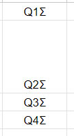
SORT(IFNA(VSTACK(data, ugc)))– vertically stacks thedatawith theugc. As the number of columns in both arrays differ, #N/A errors may occur, which are then removed using IFNA. The result is sorted, resulting in each unique group row followed by its correspondingugcrow. Assigned name:abr(added blank row).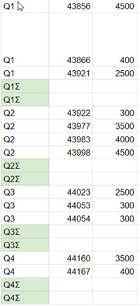
Formula Expression:
IFERROR(IF(SEARCH("Σ", abr), ""), abr) – searches for the character “Σ” in the range and replaces cells containing it with blanks.
Formula to Insert Blank Rows Between Each Group: Lambda Approach
We are utilizing REDUCE, one of the LAMBDA helper functions, to insert blank rows below each group. Specifically, the REDUCE function employs the lambda function to insert blank rows below each group, effectively separating them.
In our sample data, you can utilize the following REDUCE formula to insert one blank row below each group:
=REDUCE(
   TOCOL(,1),
   TOCOL(UNIQUE(A2:A), 1),
   LAMBDA(a, v, IFNA(VSTACK(a, FILTER(A2:C, A2:A=v),)))
)
Where:
- A2:A represents the category/group column range.
- A2:C represents the group table/data range.
To increase the number of blank rows inserted between rows, follow this pattern: VSTACK(a, FILTER(A2:C, A2:A=v),) inserts one blank row, VSTACK(a, FILTER(A2:C, A2:A=v),,) inserts two blank rows. Simply add commas to increase the number of empty rows.
Formula Explanation
Syntax of the REDUCE Function:
REDUCE(initial_value, array_or_range, lambda)Where:
initial_valueis null, represented byTOCOL(,1).array_or_rangeisTOCOL(UNIQUE(A2:A), 1), which uniques the group column A and removes any blank cells.- lambda:
LAMBDA(a, v, IFNA(VSTACK(a, FILTER(A2:C, A2:A=v),))).
Syntax of the LAMBDA Function:
LAMBDA(accumulator, current_value, calculation)In the lambda function:
a(accumulator) represents the initial value (initial_value), which is null.v(current_value) represents the current value in the array (array_or_range), initially set to “Q1”.
Here is the breakdown of the calculation part.
The FILTER formula, FILTER(A2:C, A2:A=v), filters the range A2:C based on the current value v in column A.
VSTACK vertically stacks the accumulator value (null initially) and the filtered result, followed by a comma.
This process results in the following:
| Q1 | 26-Jan-20 | 4500 |
| Q1 | 05-Feb-20 | 400 |
| Q1 | 31-Mar-20 | 2500 |
| #N/A | #N/A |
The IFNA function removes the #N/A errors. This effectively inserts a blank row below the first group.
This process is repeated for each value in the array, with the criteria in the filter being updated accordingly.
The accumulated value will be the original table with blank rows inserted below each group.


Hello, I used the formula from above, and it works for the sheet I’m working on. What if I want to add 2 rows as I’m only getting 1 row?
I just updated the tutorial to simplify the formulas. There are two types of formulas: one lambda-based and one non-lambda-based. You can choose either.
In the sample sheet, you can see a live example with two blank rows inserted below each group.
Hi Prashanth,
This is great! Is there a way to modify the formula to insert two or more blank rows between each group?
Many thanks!
Hi, Brian,
It’s possible. You require to make two changes.
1. Replace
" "with{" "," "}(appears twice in the formula)2. Replace
"offset 1"with"offset 2"Thanks so much, Prashanth! This works perfectly!
Incredibly helpful.
Thanks again!
Hi Prashanth,
Is it somehow possible to automatically insert a row when the last row is filled. So I can insert another ticker instead of having to manually right click and insert row?
Thanks!