If you need to insert a certain number of blank rows in your data, you can do so using a formula in Google Sheets.
There are a few real-world reasons why you might want to do this. For example, you could insert blank rows in every other row to make it easier to read your data. This is also useful when you want to insert an array formula in a uniquely merged cell range, as it will prevent the formula from hiding values.
In this tutorial, I will show you how to insert 2 blank rows after every row. I will also explain how to change the number of blank rows.
There are a few different ways to do this. My preferred method is to use the REDUCE formula. We will cover this formula in detail in the last part of the tutorial. But first, let’s look at another method using VLOOKUP.
In the final part of this tutorial, I will explain why it is sometimes necessary to insert blank rows using a formula in Google Sheets.
VLOOKUP Formula to Insert Blank Rows in Google Sheets
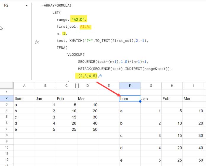
Let me first introduce you to the VLOOKUP formula that I used in cell F2. Then, I will explain what changes you may need to make to the formula to use it in your dataset. Finally, I will give a brief explanation of the formula.
=ARRAYFORMULA(
     LET(
       range, "A2:B",
       first_col, A1:A,
       n, 2,
       test, XMATCH("?*",TO_TEXT(first_col),2,-1),
       IFNA(
            VLOOKUP(
                 SEQUENCE(test*(n+1),1,0)/(n+1)+1,
                 HSTACK(SEQUENCE(test),INDIRECT(range&test)),
                 {2,3},0
            )
       )
     )
)
The above VLOOKUP formula inserts two blank rows after every other row.
How to adjust this formula for your data range?
I know your data range may be entirely different. To enable you to use this formula in a different data range/array, I need to explain what changes are required in the above formula.
1. Changing Data Range in the Formula
Assume you want to insert two blank rows after every other row in the range B5:C. You need to make the following changes in my formula:
- Replace the
rangein the formula from"A2:B"to"B5:C". - Replace
first_colin the formula fromA1:AtoB1:B. This is important. You should keep the first column (first_col) range starting from the first row, not from the 5th row.
The above formula inserts 2 rows after every row. To change the number of blank rows, you need to change the value of the n argument.
2. Changing the Number of Rows to Insert
See how simple it is to increase the number of blank rows. You replace the value of n in the formula from 2 to the number you want. In the following example, I am going to set it to 3.
The below formula inserts 3 blank rows after every alternate row in the range B5:C.
=ARRAYFORMULA(
     LET(
       range, "B5:C",
       first_col, B1:B,
       n, 3,
       test, XMATCH("?*",TO_TEXT(first_col),2,-1),
       IFNA(
            VLOOKUP(
                 SEQUENCE(test*(n+1),1,0)/(n+1)+1,
                 HSTACK(SEQUENCE(test),INDIRECT(range&test)),
                 {2,3},0
            )
       )
     )
)
3. Changing the Number of Columns
In my above examples, I have used a two-column sample data.
If you have a different number of columns, such as A2:C, then the formula part {2,3} should be changed to {2,3,4}. Similarly, if the number of columns is 4, then it will be {2, 3, 4, 5}.
If you want to learn more about this VLOOKUP array feature, check out this tutorial: Multiple Values Using Vlookup in Google Sheets is Possible [How to]
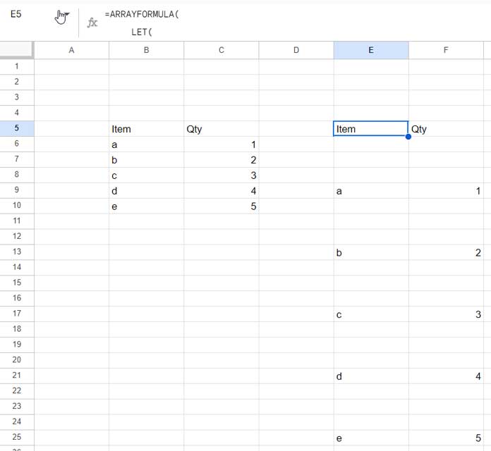
The following formula (shown in the screenshot) inserts 1 blank row after every other row in the range A2:D.
Anatomy of the VLOOKUP Formula for Inserting Blank Rows in Google Sheets
Here is the crux of the formula:
I used two SEQUENCE formulas. One was added to the range, and the other was used as the VLOOKUP search_key.
Syntax of the VLOOKUP Function in Google Sheets:
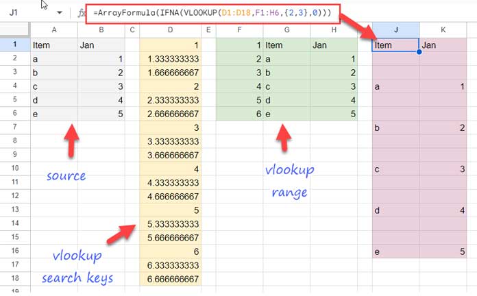
VLOOKUP(search_key, range, index, [is_sorted])Assume the data range is A1:B6. That means there are 6 records in the table.
The =SEQUENCE(6) formula will return the numbers 1 to 6, which are then stacked to the data range as follows (please refer to F1:H6 in the below image):
=HSTACK(SEQUENCE(6),A1:B6)This is the range in VLOOKUP.
Now, the search key is the sequence numbers * n / (n + 1) formula. Let’s consider n is 3, then it will be:
=ArrayFormula(SEQUENCE(6 * 3, 1, 0) / 3 + 1)Please refer to D1:D18 in the below image.
With VLOOKUP, we can now easily insert n blank rows below every other row. Please see the illustration below.
REDUCE Formula to Insert Blank Rows in Google Sheets
The above VLOOKUP is a dynamic formula that works with both open and closed ranges. We can use the REDUCE function to code a dynamic formula similar to inserting blank rows below every other row.
However, to make things simple, I will opt to use it on limited ranges.
We can use the following REDUCE formula to insert one blank row below each other row in the closed range B3:E8:
=REDUCE(,B3:B8,LAMBDA(a,v,IFNA(VSTACK(a,FILTER(B3:E8,ROW(B3:B8)=ROW(v)),))))Here,
B3:B8is the first column range in the source data.B3:E8is the source data range.
To insert two blank rows, add one more comma immediately after the last comma in the formula.
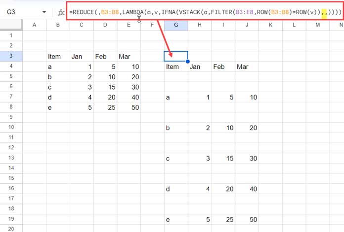
This formula has an issue. It will insert one blank row at the top, but it is the best formula to insert blank rows in Google Sheets, ignoring the closed range issue.
Formula Logic and Explanation
The FILTER function filters the first row in the range.
FILTER(B3:E8,ROW(B3:B8)=ROW(v))where v is equal to B3.
VSTACK stacks the accumulator value (a), which is blank in the first step, with the above filtered row and then a single blank cell.
VSTACK(a,FILTER(B3:E8,ROW(B3:B8)=ROW(v)),)In the next step, within VSTACK, the accumulator value will be the above result. v in FILTER(B3:E8, ROW(B3:B8) = ROW(v)) becomes B4.
This repeats until the last row in the range.
That’s the logic behind the REDUCE formula that inserts blank rows below every other row in Google Sheets.
Reveal Hidden or Trimmed Off Values in Merged Cells in Google Sheets
Have you ever tried applying an array formula to the topmost cell of a merged cell range? If so, does it correctly output all the values?
When you use an array formula in a merged cell range, it hides a certain number of values, depending on the number of rows merged.
Please see Figure 6 below for an example.
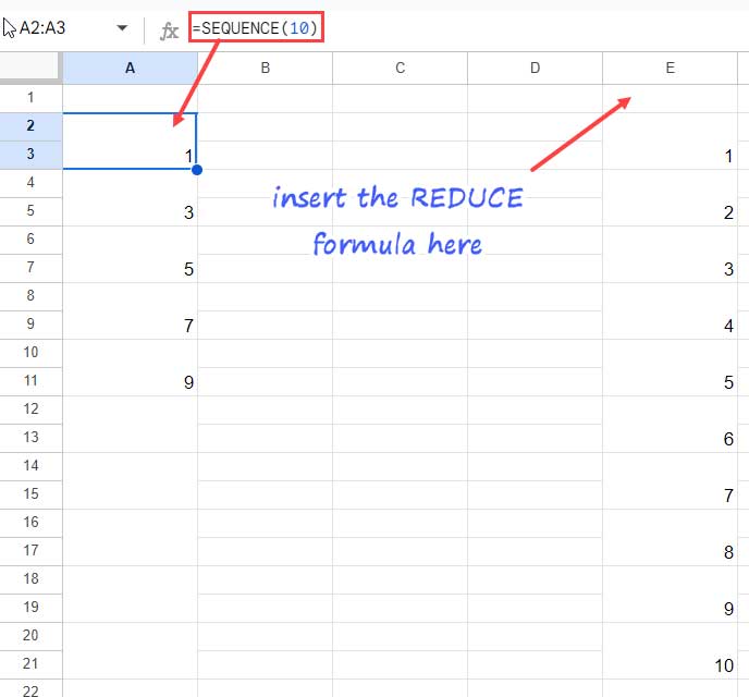
=SEQUENCE(10)You can see that the SEQUENCE formula in cell A2 does not return all the numbers from 1 to 10. Some values are hidden because of the merged cells.
You have already learned how to insert blank rows using a formula in Google Sheets. It’s time to test it in a real-life scenario.
You can pick the REDUCE-based formula. I am avoiding the VLOOKUP-based formula because it uses range as a text string (within double quotes).
=REDUCE(,A1:A10,LAMBDA(a,v,IFNA(VSTACK(a,FILTER(SEQUENCE(10),ROW(A1:A10)=ROW(v)),))))This formula in E1 will return all the values correctly. However, we should enter the formula in an unmerged cell because it returns an empty cell at the top.
The SEQUENCE formula returns 10 numbers. So we should specify A1:A10 in the formula. If the formula returns 100 numbers, then you should specify A1:A100.
If you use any other formula instead of SEQUENCE, for example, a QUERY, you must first check the number of rows the QUERY returns and specify a range accordingly, instead of A1:A100.
Note: The above formula requires uniquely merged cells to work correctly.
Related:


Here is an update! I have edited the old formula and also added a new one.
I found an interesting/frustrating phenomenon with your last example.
If the column range starts on an even row number (A2, A4, A6, etc.), it starts the spaced column one row down.
Also, in the last example, if you increase the number of rows between each cell, you have to increase the amount you multiply by
[,counta(A1:A)*2]. Otherwise, the printout column will not show the whole list.Hi, Shivaraj,
Thank you for bringing the problems to my notice, and sorry for the inconvenience caused.
Issue # 1:- Please see the new update at the bottom of the tutorial.
Issue # 2:- I assume you have interpreted it based on the screenshot but missed the update immediately below.
Hello!
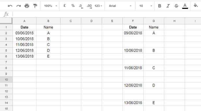
Great tutorial. Thank you for posting. Any thoughts on how to repeat text for those rows instead of them being blank? The output would look like this:
09/06/2018 A
09/06/2018 A
09/06/2018 A
01/01/2022 B
01/01/2022 B
01/01/2022 B
….
THANKS!
Hi, Astrid,
To repeat the first column.
=ArrayFormula(FLATTEN(SUBSTITUTE(filter(A2:A,$A$2:$A<>""),"",{1,2,3})))To repeat the second column.
=ArrayFormula(FLATTEN(SUBSTITUTE(filter(B2:B,$A$2:$A<>""),"",{1,2,3})))To repeat 4 times use the array {1,2,3,4} instead.
I’ve been trying for hours to replicate exactly the Vlookup example.
PLEASE! make sure to put a note to check on syntax differences while using your google sheets formulas. For instance, in my case I had to chance {2,3} by {2\3}
Hi Prashanth,
Would it be possible to include this concept with an
=query(importrange())?How would you, for example, manage if your data is coming from an external google sheet?
Hi, Martijn,
The easiest way is first to import the data into a sheet, and in another sheet within that file, you can use my SORT-based formula.
If you don’t want to import separately, you can try this with closed ranges.
Example:-
Data Range to Import: Sheet1!A1:C100
Formula:
=array_constrain(sort(importrange_formula_Sheet1!A1:C100,sort(row(A1:A100),
mod(Row(A1:A100),2),0),1),counta(importrange_formula_Sheet1!A1:A100)
*2,3)
Hi Prashanth,
Is it possible that instead of spaces in between values, you can put a different value? For example, I have a list of Appointment Types from Col A2:A and from B:H are days of the week. I want that instead of spaces in between of those appointment types, I want to put Attended, Cancelled, and Total (Total of three 3 spaces)
Hi, Spencer D,
You can explain the problem better with the help of a sample sheet. If possible, share the URL via a reply to this comment.
In the meantime, you can read this post that may help you insert total rows.
Inserting Subtotal Rows in a Query Table in Google Sheets.
I have an additional 3 rows at the top of the column when I use this formula, how do I remove them??
=array_constrain(sort(DropDowns!C2:C,sort(row(DropDowns!C2:C),mod(Row(DropDowns!C2:C),6),0),1),counta(DropDowns!C2:C)*6,1)
Hi, Elisabeth H Bent,
Sorry! I can’t correct the formula without seeing your data in use.
What you can do is, offset 3 rows using Query as per the below syntax.
=query(your_formula,"Select * offset 3",0)Hi Prashanth,
Great formula, thank you!
I’ve been able to use it to create the empty rows but I’m now wanting to extend it to populate the columns in the empty rows based on the values of the rows had values in initially.
Can I contact you directly regarding this please?
Thanks
Hi, Dave,
Please share a sheet contains some mockup data. Let me understand the problem from that. If I can solve the problem with a formula, I’ll definitely help you.
Share the link via comment (I won’t publish it).
Unfortunately, in Sheet2!b2 it says N/A and you now have full access.
Hi, Zolly,
I have copied your sheet and entered the formulas. Already sent it via email.
Hey Prashant
I can’t thank you enough…
It would take me a week to finish what I want(Ed)
Can you adjust your Answer to move all contents of each row to “move” with their respective date?
Hi, Zolly,
That seems simple. But your sheet is View only. So I am unable to enter my formula.
Please follow the below steps.
1. Copy the Sheet1 formula (in cell B2) to Sheet2!B2.
2. Delete Sheet1 column 2 (that contains my formula).
3. Empty all the values in Sheet2 except the values in columns A and B.
4. In Sheet2!C2, insert the below Vlookup.
=ArrayFormula(IFNA(vlookup(B2:B,Sheet1!A2:T,sequence(1,15,2),0)))This way you can insert blank rows, put your preferred text (day of the week) and align other columns accordingly.
If you face issues, give me “EDIT” access.
I would like to add a row after each date change.
Column A
12/5/2020 10:00:00 AM
12/5/2020 12:00:00 PM
12/5/2020 2:00:00 PM
12/5/2020 5:00:00 PM
12/7/2020 10:00:00 AM
12/7/2020 12:00:00 PM
12/7/2020 2:00:00 PM
12/7/2020 6:00:00 PM
12/8/2020 2:00:00 PM
12/8/2020 6:00:00 PM
12/9/2020 11:00:00 AM
12/9/2020 1:00:00 PM
12/9/2020 4:00:00 PM
12/9/2020 6:00:00 PM
12/10/2020 10:00:00 AM
12/10/2020 12:00:00 PM
12/10/2020 6:00:00 PM
12/12/2020 10:00:00 AM
12/12/2020 12:00:00 PM
12/12/2020 2:00:00 PM
And then I’d like to insert the day of the week in A1 of that new row.
Hi, Zolly,
I assume the above dates are in the range A2:A. If so, in B2, insert the below formula.
=ArrayFormula(if(filter(sort({A2:A;unique(int(A2:A))}),sort({A2:A;unique(int(A2:A))})<>0)-int(filter(sort({A2:A;unique(int(A2:A))}),
sort({A2:A;unique(int(A2:A))})<>0))=0,
text(filter(sort({A2:A;unique(int(A2:A))}),
sort({A2:A;unique(int(A2:A))})<>0),"ddd"),filter(sort({A2:A;unique(int(A2:A))}),
sort({A2:A;unique(int(A2:A))})<>0)))
Note:- A2:A must be date-time (timestamp).
Hey Prashanth,
Great idea to use this array formula. I am trying to use it but my case is a bit different.
In that I want to control the number of empty rows added with a cell value.
I have 6 columns and they sort of look like this:
NAME | ADDRESS | STATE | NUMBERVALUE | USERNAME | PASSWORD
John | 34 lark st. |CA | 3 | JONY555 | qwerty555
Tim | 45 poet st. | VA | 4 | TIMTIGER4 | qwerty222
Can your array dynamically insert blank rows underneath each line based on the number values in column 4 (4NUMBERVALUE)? In this example, I imagine that it will automatically insert 3 rows below “JOHN”, and 4 rows under “TIM”?
Thanks again for your great tutorial, and I hope to hear from you soon!
Hi, EJ,
I have already posted a similar tutorial here – Count Words and Insert Equivalent Blank Rows in Google Sheets.
Since you have already a ‘number’ column (column D if the range is A1:F), you can skip the step # 1 in that tutorial. Rest of the formula parts are the same.
Read that tutorial and learn to code yourself. If you want a ready-made solution, here is the formula.
Range: A1:F (A1:F1 contains the labels and the data starts from the row#2 onwards).
Insert the below formula in cell G2.
=Query(sort(iferror({{transpose(split(query(rept(row(A2:A)&" ",D2:D),,9^9)," ")),sequence(sum(D2:D),columns(A1:F1))/0};{row(A2:A),A2:F}})),"Select Col2,Col3,Col4,Col5,Col6",0)Best,
Amazing! That worked like a charm… Thank you, Prashanth! You are truly a Google Sheets WIZARD!
What if for example, I have these:
Account1
Account1
Account1
Account2
Account2
And I would like it to be like this:
Account1
Account1
Account1
Account2
Account2
May I know how to do it. I’ve modified your formula but I could not seem to do it.
Hi, Mae Noda,
I’ll check it and update you in the coming days.
Thanks.
Hi, Mae Noda,
I have written a new tutorial in which I shared the required formula and explanation.
Please check the bottom of the post.
I figured it out. The extra blank cells at the end are necessary. I had the range narrowed to just the cells I wanted.
Sorry, apparently my original comment never got posted. I do have a couple of useful things to add, though:
A way to do without the extra spaces at the end:
=array_constrain(sort({ARRAY_CONSTRAIN($A$5:$A,COUNTA($A$5:$A),1);TRANSPOSE(SPLIT(REPT("X,",COUNTA($A$5:$A)),","))},sort(row(OFFSET(
$A$5,0,0,COUNTA($A$5:$A)*2,1)),mod(Row(OFFSET($A$5,0,0,
COUNTA($A$5:$A)*2,1)),2),0),1),counta($A$5:$A)*2,1)
A way to do this horizontally:
=ARRAY_CONSTRAIN(TRANSPOSE(sort(TRANSPOSE({ARRAY_CONSTRAIN($K$1:$1,1,COUNTA($K$1:$1)),SPLIT(REPT("X,",COUNTA($K$1:$1)),",")}),
sort(TRANSPOSE(COLUMN(OFFSET($K$1,0,0,1,COUNTA($K$1:$1)*2))),
mod(TRANSPOSE(COLUMN(OFFSET($K$1,0,0,1,COUNTA($K$1:$1)*2))),2),0),
1)),1,COUNTA($K$1:$1)*2)
Thanks for sharing!
Hi Prashant,
Thank you very much. I placed the formula into cell G2. The ultimate goal was to start the formula populating the results beginning at G2 (No blank rows before the first data row). This formula results with the first data row beginning at G4.
Also, I realized the added blank rows are not editable. Anyway to insert editable blank rows?
Thanks for your help.
Jack
Hi, Jack,
Sorry for the trouble. I have updated my tutorial with more details to enable readers to easily change the formula (as well as understand) for their data range.
As you may well aware, editing an output area (range) of an array formula will break the formula. So once you have inserted the desired number of rows using my formula, copy and paste value the output into a new sheet.
Hi Prashanth,
In the section “Insert Blank Rows Using SORT Based Formula in Google Sheets”, was the formula supposed to sort and insert blank rows? From the image attached, it doesn’t look like it’s sorted. Is there a formula to sort a range B1:F and also insert blank rows?
Thanks
Jack
Hi, Jack,
The formula is not meant for sorting and inserting blank rows. If you want, it’s not difficult to achieve that. You only need to wrap the range with SORT.
Hi Prashanth,
I’m new to Google Sheets but I was wondering if it’s possible to combine your code with a “What If” statement. Basically, I am looking to create more rows by the number of words there are.
So if a cell has (banana, apple, oranges) and another cell has (grapes, soda), rather than have a fixed amount of rows in between the cells, only add 2 empty rows underneath (banana, apple, oranges) and only add one empty row underneath (grapes, soda).
Thank you!
Best,
Hi, Samuel,
I have successfully written formula for the said purpose. I’ll update you soon!
Best,
Here you go!
https://infoinspired.com/google-docs/spreadsheet/count-words-and-insert-blank-rows-in-google-sheets/
Can you write the same formula for EXCEL?
Thanks in advance.
It can be done also by
={formula1;formula2; formula3;etc...}Actually solution which you have offered it is not really a practical solution because empty rows ‘inserted’ with your formulas only look good visually but practically you cannot do anything practical with them because as soon as you try to use them by trying to enter some content into them, your formula throws an error 🙁
But, nice try 🙂
Forgive me for criticism. I just report the results of my testing. Thank you for posting them.
All the best.
Hi, Kavi Karnapura,
Thanks for your feedback!
If you use my formula to insert blank rows, if you want to add new values to the inserted rows, then you should copy-paste (paste value) the formula output to a new range.
It’s applicable to all the formula based solutions.
Best,
Dear Prashant,
I have done a little testing of your formulas which you have provided but they don’t really insert blank lines into a Google Sheet.
By inserting lines I understand that if there is some content below it gets moved down not overwritten.
I tried putting (entering) some content bellow the cell that is containing your given formula and I got an error: “Array result was not expanded because it would overwrite data in cell bellow the formula”.
I am looking for a formula that would push (move) the content bellow the formula and not throws an error if a cell bellows the formula contains some value.
So, I want to have a floating row that moves down or up according to the number of items in the list.
Is this possible to achieve?
Thank you in advance for your time and help.
Kavi…
Hi,
An array formula needs blank rows/column to expand. If any cell below the formula (formula output range) contains values, then the formula won’t work.
It might be achieved via Apps Script. For help, you can refer to this Google Apps Script community.
Best,
Dear Prashanth,
I have a seemingly easy problem but I can’t figure out how to modify your functions to solve it.
I would just like to insert one time (no arrayformula) as many blank rows as there are items in the range.
For example, you have 6 kinds of fruits listed in your range and I would like to insert 6 empty rows.
If there would be 5 kinds of fruits listed in your range, then the formula should insert 5 empty rows.
If there would be N kinds of fruits listed in your range, then the formula should insert N empty rows.
And the list of fruits is on one sheet and inserted rows should be on another sheet in the same spreadsheet.
Let’s say that the list of fruits is my shopping list what I have to buy and on the second sheet I want to do the calculation of what I bought.
So, the second sheet should contain a fixed head with pieces of information of the seller who sold me fruits and the foot where the totals (sums) would be calculated.
The second sheet should look something like this:
First row: Grocery shop XYZ, Some street address, Invoice number, date of purchase
Second row: Item’s name, item’s unit, the number of units bought, the price per unit, price of units bought
Third row: bananas, kg, 3, 1.2, 3.6
Fourth row: apples, kg, 2, 1.3, 2.6
Final row: TOTALS: total units bought: 5, total amount paid: 6.2
So, between the final row and the second row in the above example, there should be N blank rows inserted where N is the number of items in a shopping list on another sheet in the same spreadsheet.
So, basically I want to prepare space for query formula to execute and list down the items bought and on the end of query formula I want to add a row with totals.
I hope that you can understand what I am trying to achieve?
Could you please kindly help me out?
Thank you in advance.
Hi, Kavi Karnapura,
Why don’t you combine two Query formulas – One for grouping and another for a total row?
Can you share a copy (in View or Edit mode) of your Sheet? Mockup data would be enough for my testing.
Best,