Here is a simple hack to help you insert subtotal rows in a Query table in Google Sheets. You can use this method if you don’t want to use the built-in Pivot table.

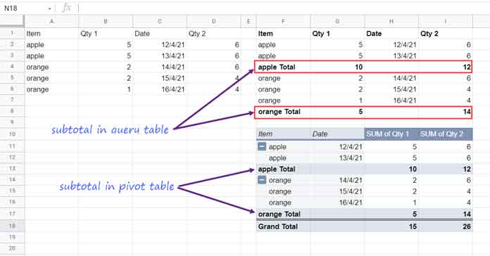
In a Pivot table, you can get totals (subtotals) and a grand total row. The total rows are for section-wise (group-wise) totals, whereas the grand total row is for the sum of section-wise totals.

Before starting to learn how to insert subtotal rows in a Query table in Google Sheets, let’s see how it compares with a Pivot table.

One of the main advantages of the Query table that contains subtotals is that it can retain the positions of the columns as per the original data. It’s flexible, so you can move the columns around. In the Pivot table, it won’t be the case.

For example, let’s compare the below two outputs – the Query table in F1:I8 and the Pivot table in F10:I18. As you can see, the Query table retains the column positions in comparison to the source data.

Note: It’s quite easy to add the grand total row to the Query table. I have already explained the same earlier (please see the ‘Resources’ section at the end of this tutorial). So, I am skipping it.

To insert subtotal rows in a Query table, we will use three Query formulas in nested form.

How to Insert Subtotal Rows in a Query Table in Google Sheets

For the sample data, please refer to the range A1:D in the screenshot above or copy my sample sheet with the formula below.

Sample_Sheet_18421

Since there are three Query formulas involved, the number of steps will also be three. Among the three, the second Query formula is the most important one as it generates subtotal rows to insert.

The first and second Queries will generate two tables. The purpose of the third Query is to combine them properly.

Related: How to Combine Two Query Results in Google Sheets.

None of the below formulas are complicated. If you face any issues, you may think about spending some of your leisure time learning Query.

Must Check: Google Sheets Function Guide [Quickly Learn Popular Functions].

Step 1: Select Columns and Remove Blanks (Table 1)

This step is not directly related to subtotal rows, but it is a crucial part of the formula for inserting subtotal rows in a Query table.

Insert this formula in cell F1. It will return the table in the range A1:D as it is.

=QUERY(A1:D, "SELECT A, B, C, D WHERE A IS NOT NULL", 1)

There are four columns in my table: Item, Qty 1, Date, and Qty 2.

I am selecting all the columns. If you want, you can choose only the columns that you want. You can also change the column positions.

If you want to skip or change column positions, do the same by modifying the formula part A, B, C, D in the SELECT clause of Query.

For example, to select Item, Qty1, and Qty 2, replace A, B, C, D with A, B, D.

Depending on this change, there will be adjustments in the step 2 formula below. So, for the time being, stick with my above formula. Once learned, you may adjust the columns.

As I have already mentioned, the purpose of the above formula is to return the required columns and eliminate any blank rows.

Now, let’s shift our attention to the step 2 formula below, which is the key to inserting subtotal rows in a Query table in Google Sheets.

Step 2: Key Formula to Generate Subtotal Rows (Table 2)

The formula below goes in cell F8. We will combine the formulas in cells F1 and F8 in the final step.

=QUERY(ArrayFormula(IF(LEN(A2:A), {A2:A&" Total", B2:D},)), "SELECT Col1, SUM(Col2), ' ', SUM(Col4) WHERE Col1 IS NOT NULL GROUP BY Col1 LABEL SUM(Col2) '', SUM(Col4) '',' '''")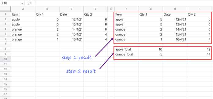

As you can see, it returns the subtotal rows to insert in the Query table.

In the third step, we will combine the results from steps 1 and 2 vertically and then sort column 1 in ascending order. This way, we can insert subtotal rows in a Query table in Google Sheets.

Before proceeding to the final step, let’s spend some time understanding the formula used in step 2.

I know I should explain the formula here in detail. Let me start with the QUERY function syntax and then the formula.

QUERY(data, query, [headers])

There are three arguments. Let’s see how each one of them contributes to the formula.

Data Part:

In the above formula, the data is ArrayFormula(IF(LEN(A2:A), {A2:A&" Total", B2:D},)).

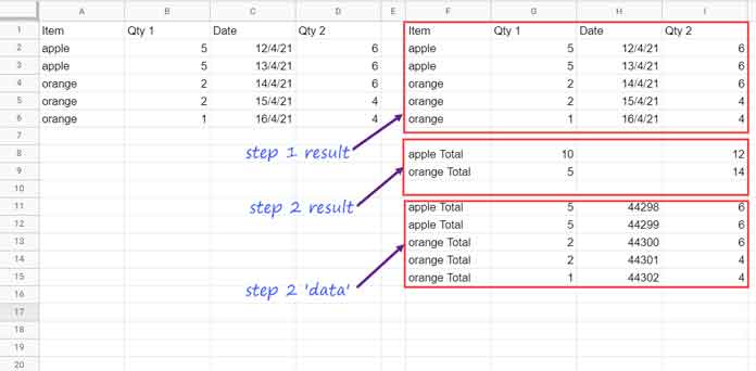
It simply returns the source data in A1:D as it is. The only change is it adds the text “Total” at the end of the values (items) in A2:A.

That means all the text for ‘apple’ will become ‘apple Total’ and all the text for ‘orange’ will become ‘orange Total’. Please refer to F11:I15.

Let me elaborate on the formula further as it plays a vital role in inserting subtotal rows in the Query table in Google Sheets. But feel free to jump to the next subtitle below.

The Query ‘data’ is an IF logical test.

Syntax: IF(logical_expression, value_if_true, value_if_false)

Note: We must use the ArrayFormula function with this logical test as it uses a range, i.e., A2:A.

The logical_expression is the formula LEN(A2:A). It identifies the non-blank cells by calculating the length of characters.

If LEN(A2:A) returns numbers, that means, such cells have values. This formula tests whether there are values in the range A2:A.

The value_if_true (TRUE) in the IF logical test is {A2:A&" Total", B2:D}. We have not used the value_if_false (FALSE).

Query Part:

The Query part is as follows to summarize the ‘data’ above.

"SELECT Col1, SUM(Col2), ' ', SUM(Col4) WHERE Col1 IS NOT NULL GROUP BY Col1 LABEL SUM(Col2) '', SUM(Col4) '',' '''"

It returns column 1 (Item), sums column 2 (Qty 1), returns a blank column instead of the “Date” column, and sums column 4 (Qty 2). Further, it groups column 1.

Please see image #1. You can observe that, in the subtotal rows, which we have inserted, the cells in the “Date” column are blank. There are values in other columns in the subtotal row.

We have used ' ' to insert a blank column. You can find more details on that here – How to Insert Blank Columns In Google Sheets Query.

Header Part:

We didn’t use the header part. Our “data” in the above case has no header row.

We can either use 0 or leave the header blank to let the Query detect it automatically. I have opted for the latter.

Step 3: Insert Subtotal Rows in the Query Table by Combining Tables 1 and 2

In the third Query formula, the ‘data’ is the vertically combined step 1 and 2 tables. That means the step 2 table is placed below the step 1 table.

=QUERY(VSTACK(step_1_formula, step_2_formula),"ORDER BY Col1", 1)

The step 3 formula is only for vertically appending the two tables and then sorting column 1 (item) in ascending order. It will insert the subtotal rows below each section (each item).

Here is the final formula that inserts subtotals into the table.

=QUERY(
     VSTACK(
          QUERY(A1:D, "SELECT A, B, C, D WHERE A IS NOT NULL", 1), 
          QUERY(ArrayFormula(IF(LEN(A2:A), {A2:A&" Total", B2:D},)), 
             "SELECT Col1, SUM(Col2), ' ', SUM(Col4) WHERE Col1 IS NOT NULL 
              GROUP BY Col1 LABEL SUM(Col2) '', SUM(Col4) '',' '''"
          )
     ),"ORDER BY Col1", 1
)

Resources

We have seen how to insert subtotals in a Query table in Google Sheets. The above is the easier way to place subtotals below each group in a range.

Here are some similar tutorials.

1. In Google Sheets How to Total Each Change in a Column Value
2. Grouping and Subtotal in Google Sheets and Excel
3. Formula to Insert Group Total Rows in Google Sheets
4. Automatically Add Total to Filtered Data in Google Sheets