I am badly missing the Excel-like grouping and subtotal functionality in Google Sheets. I am sure that sooner or later Google will implement this feature in Google Spreadsheets.

In the meantime, we should find some workarounds to replicate the Excel-like grouping and subtotal in Google Sheets.

I have one solution that uses the SUMIF spreadsheet formula and the row grouping feature that Google added recently.

Grouping and Subtotal in Spreadsheets

In Excel, this grouping and subtotal functionality is built-in and named Subtotal (not the Subtotal function).

It helps users to total several rows of related data (groups of data) by automatically inserting subtotals.

In this type of subtotaling in Excel, you have the freedom to choose the total to appear at each change in your preferred column, and also the aggregation function to use (sum, average, count, etc.).

Let me show you how to group and subtotal in Excel first. This will give you a clear picture of what this topic is about.

Sample Data for Subtotal and Grouping in Google Sheets and Excel

The following is the sample data that I am using in the below examples in both Excel and Google Sheets.

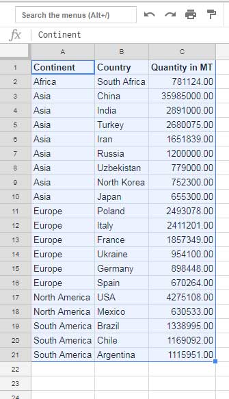
This is my sample data for row grouping and subtotaling. The data is sorted by Column A, and that is necessary. This is because my grouping of data is based on Column A, i.e., by continent names.

The list shows the world’s 20 largest apple-producing countries and their production in metric tons (MT). I am not mentioning the year of production, and I am also not confirming the authenticity of the data. This is just for our example purpose only.

Excel Grouping and Subtotal Example

In this part, I am focussing on Excel to make you understand what is row grouping and subtotal.

Steps:

1. Select the data in the range A1:C21.
2. Click on the Data menu and Select Subtotal in the Outline group.
3. Follow the below settings and click OK.

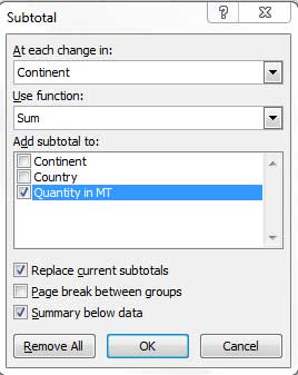
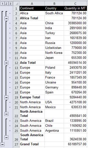
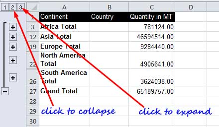
That’s all you need to do in Excel. You can now collapse the row grouping, and it will look like this:

Grouped Excel Data (expanded view by default):

Collapsed Excel Data:

The subtotal and grouping features are easy to implement in Excel since they are built-in. What about Google Sheets?

Grouping and Subtotal in Google Sheets

I will guide you on how to do grouping and subtotaling in Google Sheets, which includes some workarounds.

As mentioned, I will use the SUMIF function, and then the newly added row grouping to achieve this.

First of all, see how this subtotal and grouping (my workaround) works in Google Sheets.

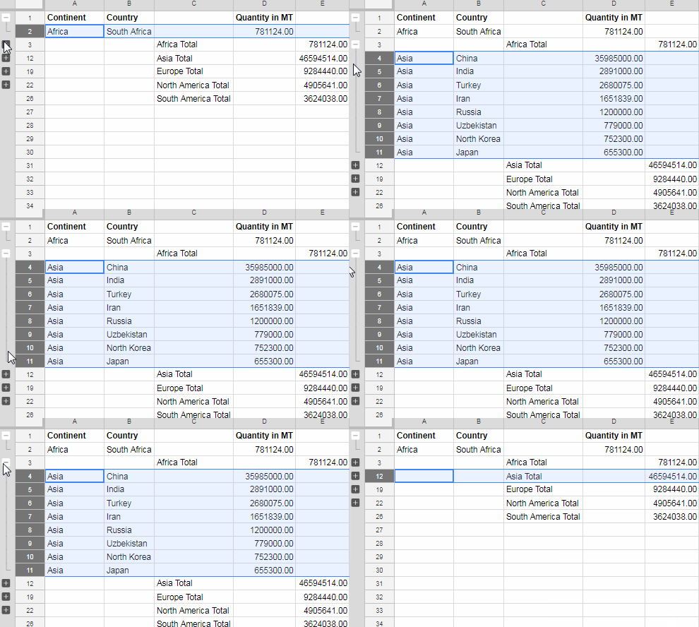
Let’s begin.

The following steps include some manual row inserting and helper columns. You can skip the row inserting if you use one of my Named Functions. We will come to that later on in this tutorial.

Note: The sample data is the same as what I used in the Excel example.

Steps involved in Subtotal and Grouping in Google Sheets

1. Insert new rows below each group. You can see the newly inserted rows in the image below (rows #3, 12, 19, 22, and 26).

2. Then, insert one helper column after column B and type the text strings as per the screenshot below (column C) in those rows.

3. Here is the SUMIF array formula that can populate subtotals in Google Sheets. You should apply this formula in cell E3 only.

Grouping and Subtotal Formula:

=ArrayFormula(if(len(A2:A),sumif(A2:A&" Total",C3:C,D2:D),))

Do not drag or copy down this formula. It will automatically expand. You only need to empty the range E3:E before inserting this SUMIF formula.

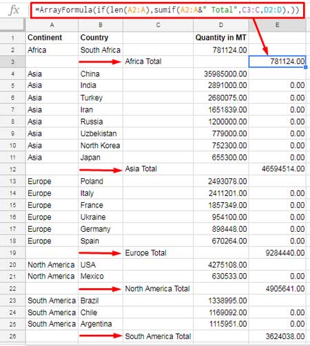
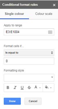
In column E, the SUMIF formula returns the group-wise (continent-wise) total of apple (fruit) production. However, there are blank cells and cells with 0 (zero) values. To remove those unwanted zeroes, we can apply a conditional formatting rule.

4. Select the range E3:E and then in Format > Conditional formatting, set the rule as follows:

If you falter with this, here is the detailed tutorial: Two Ways to Remove 0 Values in Google Sheets.

We have now reached the final part of grouping and subtotaling in Google Sheets. I mean, we have now a subtotal for each group. The only thing left to do is row grouping. Here is how to do that.

5. Select the entire row A2 by right-clicking on the row number. From the opened shortcut menu, select “View more row actions” > “Group row”.

Then, select rows 4 to 11. To do this, go to any cell in row # 4 and then press and hold the Shift key while clicking on row # 11. Finally, right-click to open the shortcut menu and apply the grouping.

Follow this grouping for all the groups, namely rows 13 to 18, 20 to 21, and 23 to 25.

Must Check: How to Group Rows and Columns in Google Sheets.

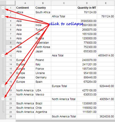
That’s it! You have now completed the grouping and subtotaling in Google Sheets.

Get My Sample Sheet

Conclusion

I know this is not a perfect solution, as it requires some row inserting and an additional helper column. However, the output somewhat mimics Excel Subtotal.

If you only want to place the subtotal at the first or last row of each group, you can simply use my AT_EACH_CHANGE named function. One of the advantages of this custom function is that you can insert average, count, min, max, etc., in addition to sum.

I hope Google will include a built-in Subtotal data menu option in Sheets in the near future.

Related Resources:-

• SUBTOTAL Function in Google Sheets: A Complete Guide.
• Formula to Insert Group Total Rows in Google Sheets.
• Blank Cell between Two Totals in Query Total Row in Google Sheets.
• Inserting Subtotal Rows in a Query Table in Google Sheets.
• How to Subtotal Up to the First Blank Cell in a Column in Google Sheets.