Do you know how to remove 0 values in Google Sheets? If not this tutorial is for you. If you are familiar with Excel you may know how to do it in Excel Spreadsheets. There is a default menu option for that. But here in Google Sheets, it’s not available.
In Excel Spreadsheet, you can do it from the file menu like File > Options > Advanced and remove the tick mark in front of “Show a zero in cells that have zero values”. It will hide all the zero values in that Spreadsheet.
If you want to remove the zeros from selected cells the above options are not suitable. Then there are two alternative methods. They are using conditional formatting and custom number format.
These two methods we can use it in Google Sheets also. Here are that two ways to remove 0 values in Google Sheets.
How to Remove 0 Values in Google Sheets
Let me start with the Customs Number format. To remove or hide zero values using the custom number format follow the below steps in Google Sheets.
1. Hide or Remove Zero Values Using Number Formatting
1. Select the cell containing the zero values. You can select few cells, or an entire range containing rows and columns.
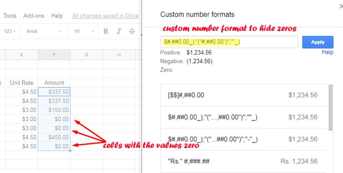
2. Then go to the menu format > number > more formats > custom number format.
3. There enter the below custom number format in the provided field and “Apply”. This instantly hides the zeros in that range.
$#,##0.00_);"("#,##0.00")";""_)

If you want to hide zeros and show a hyphen instead, you can follow the below number format.
$#,##0.00_);"("#,##0.00")";"-"_)
This will replace the zero values in Google Sheets with hyphens. Please note that the actual content in the cell will be zero.
I know it’s not possible for you to remember this format. So you may either bookmark this page or take a photo of this code using your mobile. So that you can quickly refer this setting.
From the title of this post, you can understand that there are two ways to remove the 0 values. Here is that second method.
2. Hide or Remove Zero Values in Google Sheets Using Conditional Formatting
This method is also suggestible. But it has a shortfall. I will come to that. First, see how to hide zero values with the help of conditional formatting in Google Doc Sheets.
1. Select the column or data range where the rule to be applied.
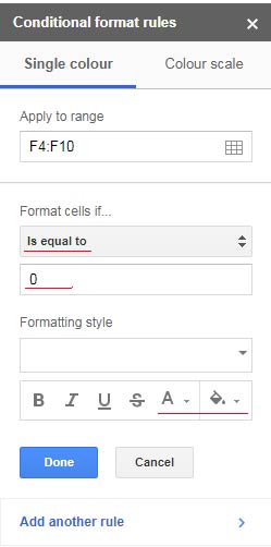
2. Go to the menu format > conditional formatting.
3. Set the conditional formatting rules as per the below image. Please ignore the “Apply to range” reference F4: F10. It should be your selected range.

Here make the font color white and set the fill color to none. Then click “Done”. This will also hide zeros.
The drawback here is you can’t change the font color or highlight the cells in the selected range later. Doing so will unhide or reveal the zeros.
That’s all. This way you can make zero values hidden in Google Doc Spreadsheets.


Great tip! The choice of methods is head & shoulders better than other answers on the interwebs, and Bob L’s addition (if the cell is a formula) is the cherry on top. Bookmarking your site.
Hi, deB,
Thanks for your feedback.
I’m not a fan of using custom or conditional formatting to create blank cells. My preference is formulas.
If the cell you’re dealing with is not a manually entered cell but has a formula you can do this:
Original Formula:
SUM(A1:A10)=IF(SUM(A1:A10)=0,"-",SUM(A1:A10))I prefer blank cells, so I just use
""rather than"-"Thank you so much for this! You’re a lifesaver.
Thanks for this. Very helpful. However, I think you’re missing the $ from the negative number format. Shouldn’t it be $#,##0.00_);”(“$#,##0.00″)”;””_)? You can see in your screenshot, you’re positive shows up as $1,234.56 while your negative number will show up as(1,234.56).