You can use a custom conditional formatting rule involving the AND and MINIFS functions to highlight the min value while excluding zeros and blank cells in Google Sheets.
If you want to include zeros but exclude blanks, you can use the MIN function with AND. I’ll share that formula as well.
The highlight rule will vary slightly depending on whether you want to apply it to a column or a row. You’ll need to use absolute and relative references appropriately for each case.
Highlight Min Excluding Zeros and Blanks in a Column
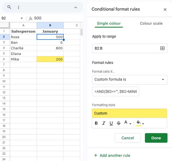
Assume you have sales figures in a column for a specific month, where each row represents a salesperson. Blank cells represent incomplete data, and zeros represent no sales.
The data structure is as follows:
- Names in column A
- Sales quantities in column B
To highlight the minimum value in B2:B, excluding blanks and zeros, follow these steps:
- Select B2:B.
- Click Format > Conditional Formatting.
- Under the Format Rules, choose Custom Formula.
- Enter the following formula:
=AND($B2<>"", $B2=MINIFS($B$2:$B, $B$2:$B, ">0")) - Choose a fill color under Formatting Style.
- Click Done.
Explanation:
The formula uses the AND function to combine conditions:
$B2<>"": Excludes empty cells.$B2=MINIFS($B$2:$B, $B$2:$B, ">0"): Ensures the value is the minimum among non-zero values in the range.
If both conditions are met, the cell will be highlighted. This logic is applied to each row individually.
Q&A
Q1: I want to find the minimum value excluding blanks in one column and highlight the entire row. What changes should I make?
A1: You don’t need to change the custom rule. Just adjust the Apply to range in the conditional formatting panel. For example, to highlight rows across A2:Z, specify A2:Z as the Apply to range instead of just B2:B.
Q2: What if I want to include zeros but exclude blanks?
A2: Replace the MINIFS formula with the MIN formula:
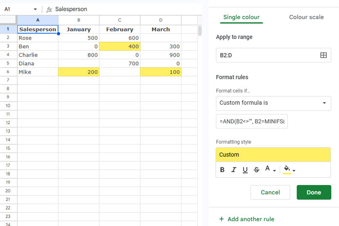
=AND($B2<>"", $B2=MIN($B$2:$B))Q3: I have monthly sales figures in columns B, C, and D. How can I highlight the minimum value in each column?
A3: Use these formulas for the Apply to range B2:D:
- Min excluding zeros and blanks:
=AND(B2<>"", B2=MINIFS(B$2:B, B$2:B, ">0")) - Min excluding blanks:
=AND(B2<>"", B2=MIN(B$2:B))
Highlight Min Excluding Zeros and Blanks in a Row
Conditional formatting isn’t limited to vertical datasets. You can evaluate values across rows and highlight accordingly.
Example:
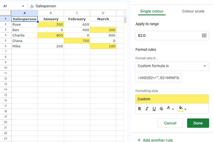
If you want to highlight the minimum sales figures for the employee “Rose” in B2:D2 (representing sales for January, February, and March), use this formula:
=AND(B2<>"", B2=MINIFS($B2:$D2, $B2:$D2, ">0"))Extending the Rule to All Rows:
To apply this rule across all rows (e.g., B2:D for all employees):
- Use B2:D as the Apply to range in the conditional formatting panel.
- Use the same formula.
Including Zeros:
To include zeros but exclude blanks, use this formula:
=AND(B2<>"", B2=MIN($B2:$D2))Conclusion
This guide demonstrates how to highlight the minimum value in Google Sheets while excluding zeros and blanks, using both column-based and row-based data structures. These conditional formatting rules can be adapted to various scenarios, ensuring your spreadsheet highlights relevant data effectively.
For a complete set of 80+ practical tutorials on Conditional Formatting, explore the full hub: The Ultimate Guide to Conditional Formatting in Google Sheets — your one-stop resource for mastering all aspects of conditional formatting.


