In Google Sheets formulas, cell references can be either relative or absolute, with the use of dollar symbols ($) influencing their behavior.
Beyond formulas in cells, these references are commonly encountered in conditional formatting. While you may also encounter them in data validation, Pivot table filter, and Data > Create a filter, their usage in these contexts is minimal.
This tutorial comprehensively covers the nuances of relative and absolute cell references in Google Sheets formulas, emphasizing the role of dollar symbols with cell references.
In Google Sheets cell formulas:
- If a cell reference is relative, it adjusts when the formula is copied to other cells.
- If a cell reference is absolute, it remains unchanged when the formula is copied.
In Google Sheets conditional formatting:
- If a cell reference is relative, it adjusts with the cells in the ‘Apply to range.’
- If a cell reference is absolute, it remains constant in the cells within the ‘Apply to range.’
There are three different ways to use dollar symbols in a formula to lock cell references:
- Both column and row are absolute.
- The column is absolute, row is relative.
- The row is absolute, column is relative.
Let’s unravel the details step by step.
Introduction to Relative and Absolute Cell References in Formulas in Google Sheets
A cell reference is essentially a cell address, comprising a column letter and row number. Each cell in the grid has a unique identifier known as a cell reference.
By default, a cell reference is relative. When used in formulas and copied to other cells, the reference automatically adjusts the column letter and row number relative to the current position.
To lock a cell reference (create an absolute reference) to a specific cell, you need to use two dollar symbols: one preceding the column letter and the other preceding the row number.
It’s possible to make either the column or the row absolute, and correct placement of dollar symbols with cell references in formulas is crucial.
Examples of Relative Cell References in Google Sheets Formulas
Relative Cell Reference in a Formula Copied to Cells Down:
In the following example, I’ve employed the formula =ROW(A1) in cell A2 to retrieve the row number.
It will return 1, representing the row number of cell A1 in A2.
If I copy and paste this formula into cell A3, it will return 2 because the cell reference becomes A2:
=ROW(A2)Similarly, if I paste the formula in cell A10, it will return 9:
=ROW(A9)
Relative Cell Reference in a Formula Copied to Cells Across:
If we copy-paste the A2 formula into cell B2, the formula becomes =ROW(B1), and the result will be one since the formula is in the same row. The ROW function returns the row number.
Let’s try a different formula this time, utilizing the COLUMN function that returns the column number.
In cell A2, enter =COLUMN(A1) and copy-paste it across. It will become COLUMN(B1), COLUMN(C1), and so on. The result will be the numbers 1, 2, 3.
If you copy the formula in cell A2, which is =COLUMN(A1), to cell B10, the formula will become =COLUMN(B9).
Using Dollar Symbols in Formulas to Convert Relative Cell References to Absolute
Here is an example of an absolute cell reference by placing dollar symbols within cell references in Google Sheets.
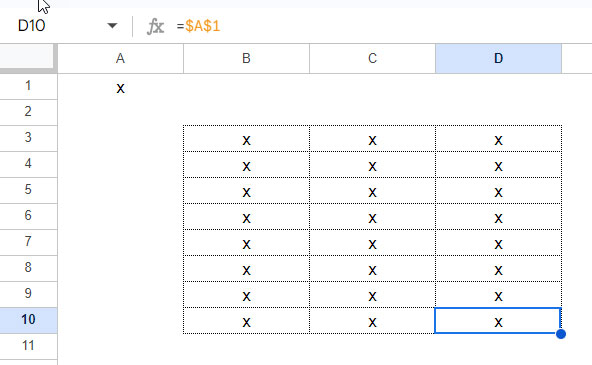
Both Column and Row are Absolute:
Cell A1 contains an “x” mark. Enter the following formula in cell B3 and copy-paste the formula to cells B4:B10 and C3:D10.
The formula will place the “x” mark in all the cells in the range B3:D10, as the formula in all the cells will be the same.
Mixed References:
In the following examples, I have the formula in cell C2 where the column in the first cell reference is absolute, and the row in the second cell reference is absolute.
=$B2*C$1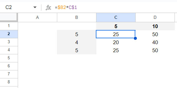
Let’s see what happens when we copy-paste this formula down and across.
When I copy this formula down, the $B2 becomes $B3 and $B4, but C$1 remains the same. So the formulas in C2:C5 will be:
=$B2*C$1 // in C2
=$B3*C$1 // in C3
=$B4*C$1 // in C4
If you copy and paste these three formulas into D2:D5, it will be as follows:
=$B2*D$1 // in D2
=$B3*D$1 // in D3
=$B4*D$1 // in D4
The above formulas are designed to help you understand how to use dollar symbols to convert relative cell references into absolute ones, either fully or partially.
In real life, you can clear cells C2:D4 and use the following MMULT to perform matrix multiplication on two matrices: B2:B4 and C1:D1.
=MMULT(B2:B4, C1:D1)Conclusion
We have learned how to use dollar symbols with formulas to obtain both relative and absolute cell references in Google Sheets.
Their significance extends to conditional formatting as well. You can gain a deeper understanding by referring to my following two tutorials:


