You can now unlock rows and columns in the data validation “List from a range” drop-down menu. It is called relative reference in a drop-down menu in Google Sheets.
Earlier the reference in the drop-down was locked by default. That means Google Sheets was only supporting absolute references by default.
What is the benefit of this new update?
Suppose I have a drop-down menu in cell E10. When I click the drop-down in cell E10, I will see a list of items to select.
If I have created the drop-down using the “List from a range” not “List of items”, with the new update, we can decide whether to change the list when we copy the drop-down to another cell.
As a side note, “List from a range” and “List of items” are two types of lists that the drop-down in Google Sheets supports.
The former uses a list from a cell range, whereas the latter uses a comma-separated list as values within the drop-down menu field itself.
The new unlock rows and columns feature makes my multi-row dependent drop-down list much more flexible and useful.
Let’s learn more about relative reference in drop-down menu in Google Sheets.
How to Use Relative and Absolute References in Drop-Down in Google Sheets
The below two examples will help you learn the use of relative and absolute references in the data validation “List from a range” drop-down in Google Sheets.
Absolute Reference (Locked Rows and Columns) in List From a Range
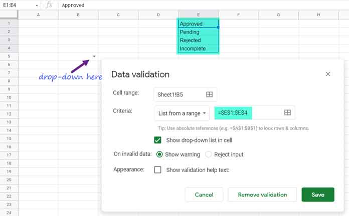
In a blank Google Sheets, let’s create a drop-down menu in cell B5. For that, we require a list. Here is it to use in E1:E4.
I have got the following values in E1:E4.
| Approved |
| Pending |
| Rejected |
| Incomplete |
Click on cell B5. Then click on the menu “Data” and then click on “Data validation”. It’ll open the below window (please see the image below).
Click the field containing “Enter a range or formula” which is the field against the Criteria “List from a range”. Then select the range E1:E4.
We want to get an absolute reference, not a relative reference, in the Drop-Down Menu. So change E1:E4 to =$E$1:$E$4.

Click “Save”.
Note:- At present, even if you do not change E1:E4 and click “Save”, Google Sheets will convert it to =$E$1:$E$4.
Now you have a drop-down in cell B5 that contains the list “Approved”, “Pending”, “Rejected”, and “Incomplete” to select.
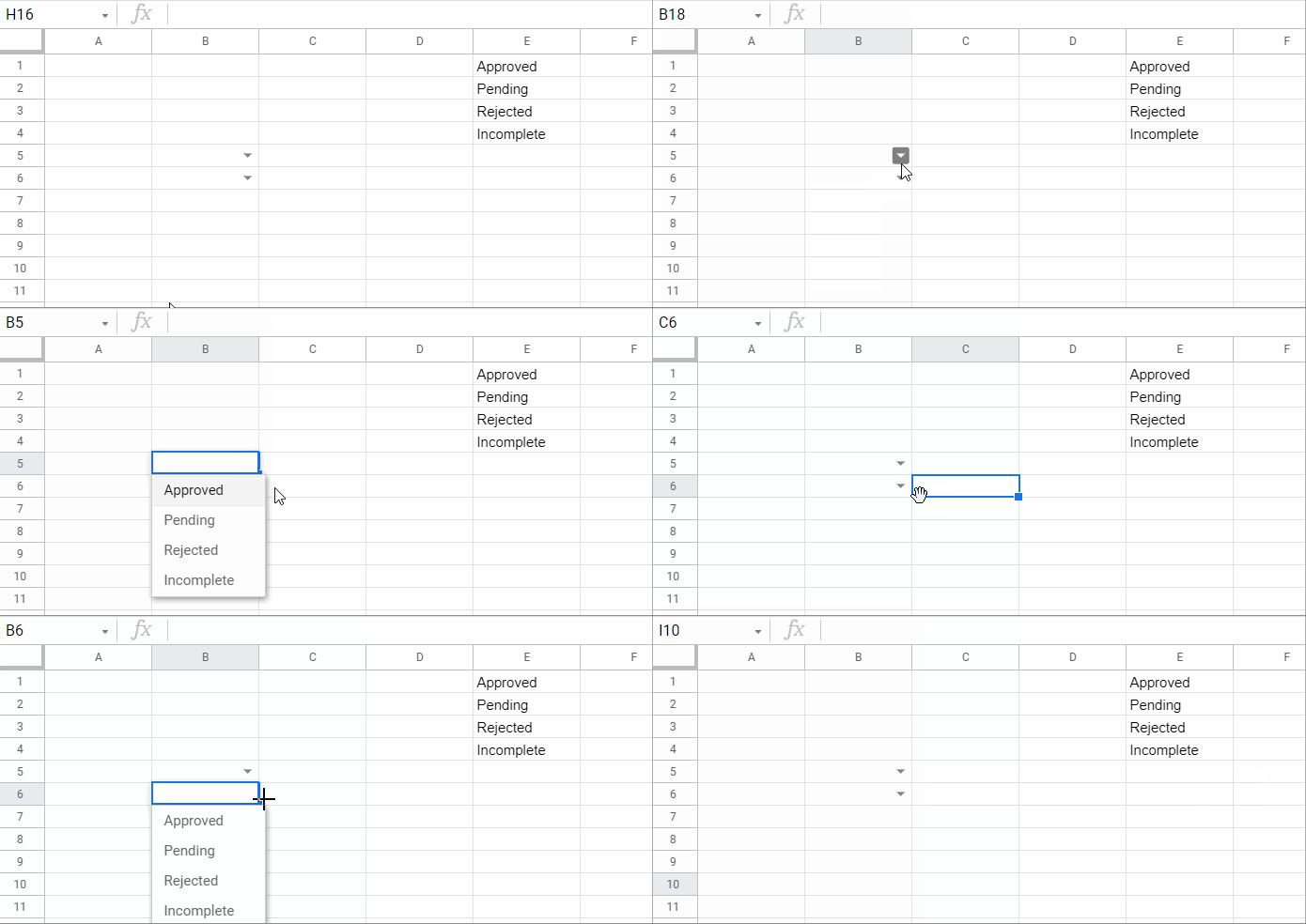
Right-click on cell B5. Then select “Copy” in the short-cut menu.
Then right-click on cell B6 and “Paste”
Check both the drop-downs. You can see that both contain the same list.

What’s the reason?
The reference in the drop-down in cell B5 is not changing when you copy it to cell B6. You can check it by opening the cell B6 drop-down in Data validation.
It is called locked rows and columns (absolute reference) in the drop-down.
Relative Reference (Unlocked Rows and Columns) in List from a Range
This part explains how to get the relative reference (unlocked rows and columns) in a drop-down menu in Google Sheets.
I want to change the reference when I copy and paste the drop-down into another cell or drag it down. Let’s see how to do that.
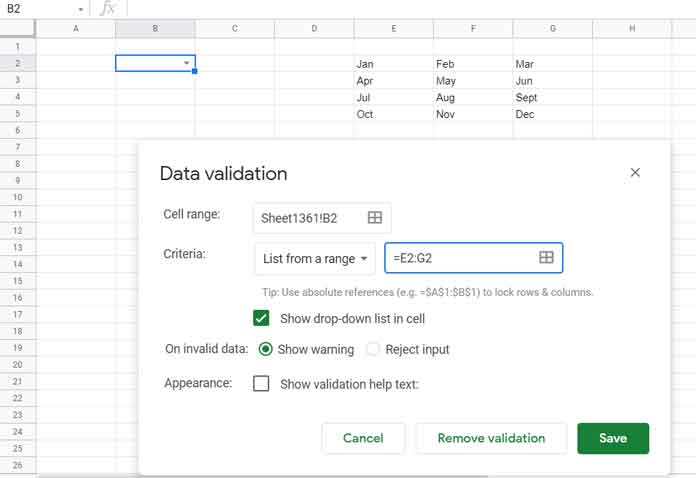
This time the range E2:G5 has the following horizontal lists.
| Jan | Feb | Mar |
| Apr | May | Jun |
| Jul | Aug | Sept |
| Oct | Nov | Dec |
In cell B2 let’s create the drop-down menu as below.

In the field against “List from a range”, the reference must be =E2:G2, not mere E2:G2.
If you use the reference without the equal sign, Sheets may convert it to absolute.
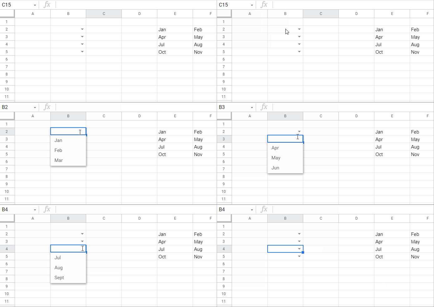
Copy-paste B2 drop down to B3, B4, and B5.

Now when you check, you can see that each drop-down has a different list from range.
The “List from a range” will be as follows.
B2 =E2:G2
B3 =E3:G3
B4 =E4:G4
B5 =E5:G5
This way, we can get a relative reference in a drop-down menu in Google Sheets.
That’s all. Enjoy!


