You can use a combination of the IF and LARGE functions to highlight the top 2 values based on a condition in Google Sheets. This method works for single or multiple conditions and is especially useful in scenarios such as:

• Highlighting the top 2 vendors from a specific country
• Highlighting the top 2 performers in a specific year

Once you understand the logic, you can easily adapt this to highlight the top 3 or even the top n values based on a condition, as this method uses the LARGE function.

Formula to Highlight the Top 2 Values Based on a Condition

=ARRAYFORMULA(
   AND(
      A1=criterion, 
      B1>=LARGE(IF($A$1:$A$1000=criterion, $B$1:$B$1000, 0), n)
   )
)

Explanation:

• $A$1:$A$1000 – Criteria range
• $B$1:$B$1000 – Value range
• criterion – The condition to evaluate
• A1 – The current cell in the criteria range
• B1 – The current cell in the value range
• n – Set to 2 to highlight the top 2 values

Formula Logic:

• The IF function checks each value in the criteria range against the condition.
• If the condition is met, it returns the corresponding value from the value range; otherwise, it returns 0.
• The LARGE function then identifies the nth largest value from the results.
• The AND function returns TRUE only if the current row matches the criterion and is one of the top n values.

This approach allows you to highlight top 2 values based on a condition in Google Sheets dynamically, without running into errors when fewer than two values match the condition.

Example: Highlight the Top 2 Sales Based on Region

In the following dataset, columns A to C represent product names, regions, and sales figures.

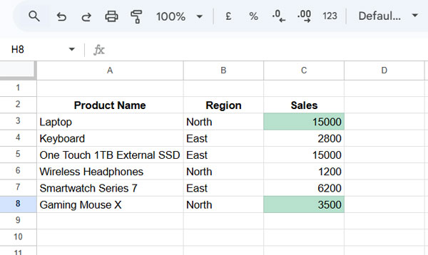
To highlight the top 2 sales in the North region, use the following custom formula in conditional formatting:

=ARRAYFORMULA(
   AND(
      B3="North", 
      C3>=LARGE(IF($B$3:$B$8="North", $C$3:$C$8, 0), 2)
   )
)

Steps to Apply the Rule

1. Select the range C3:C8.
2. Go to Format > Conditional formatting.
3. Under Format cells if, choose Custom formula is.
4. Enter the formula above.
5. Choose a formatting style.
6. Click Done.

This will highlight the top 2 values based on a condition in Google Sheets — in this case, the region “North.”

Adding Multiple Conditions

What if you want to highlight the top 2 sales from either the North or East region?

Update the formula as follows:

=ARRAYFORMULA(
   AND(
      OR(B3="North", B3="East"), 
      C3>=LARGE(IF(($B$3:$B$8="North")+($B$3:$B$8="East"), $C$3:$C$8, 0), 2)
   )
)

This updated formula uses the IF function to evaluate multiple conditions by adding logical results.

Related Resources

• How to Highlight Max Value in a Row in Google Sheets
• Google Sheets – Highlight the Max Value in Each Group
• Highlight Max Value Leaving Duplicates in Row-Wise in Google Sheets
• MAXIFS Function in Google Sheets: Find Maximum Value Conditionally
• Conditional LARGE in Google Sheets
• Highlight Largest 3 Values in Each Row in Google Sheets (+ Ties)