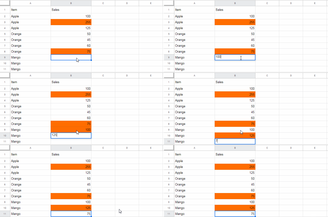
How to automatically highlight the max value in each group in Google Sheets?
If it seems tough to write a formula yourself, don’t worry! This post has the answer/solution. I have the formula to use in Google Sheets conditional formatting to conditional format the max value in each group (group-wise).
With the formula rule, we can change the cell color, font color or strike-through the max value group-wise.
Where we can use this type of cell formatting?
Here are a few scenarios.
Assume you are getting multiple Form entry on each day. With this rule, you can highlight the last form submission on each day using the timestamp column.
I mean grouping will be based on the timestamp column as well as the max value column will also be the timestamp column.
Another scenario is the sales report. In a combined sales report, we can find the salesperson who has the maximum sales volume in his name on each date.
Here we will group the data based on the date column and highlight the sales volume column (max value column).
In a dataset related to some of the sports events, for example, a car race, we can highlight who was leading in each lap of the race.
That means it’s a nice idea to learn how to highlight the max value in each group.
For your info, I am using my testing in a very basic dataset. But you can adjust the same for your real-life use. That tips also included.
Automatically Highlight the Max Value in Each Group in Google Sheets
I have used my conditional format rules in the range B2:B. See the rules (there are two rules) highlight the max values based on items (group column is column A).

I have used two custom formula rules for this. The first one is for keeping the blank cells in column B unformatted by the second rule which is the key rule.
Rule # 1:
=isblank($B2)=trueRule # 2:
The key rule which automatically highlights max in each group in your Google Sheets file.
=isna(vlookup(A2&B2,ArrayFormula(index(sortn(sort({$A$2:$A,$B$2:$B},1,0,2,0),9^9,2,1,0),0,1)&index(sortn(sort({$A$2:$A,$B$2:$B},1,0,2,0),9^9,2,1,0),0,2)),1,0))=falseI know you badly want to know how to use this formula in your Google Sheets file to conditional format max values group wise.
Further, a few of you might want to know the formula explanation as well as the logic. So here we go!
How to Apply Formulas as Conditional Format Rules in Google Sheets
Let’s talk about applying the above two rules. That will also help you to learn how to apply formulas as custom rules in conditional formatting.
The first and important thing is the custom rule order. If you are using custom rules (more than one formulas), do keep their ‘provided’ order!
Steps:
Select the range B2:B. I mean from B2 to the last cell in that column. In my sheet, it’s B2:B11.
Then we can open the conditional formatting sidebar panel from the menu Format > Conditional formatting.
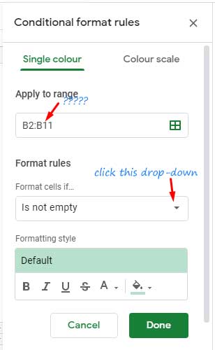
Since you have selected B2:B11 as the range, the default settings will be something like below.

This raises a question. Can’t we use an infinite range in conditional formatting in Google Sheets?
Yes! Of course. To select an infinite range, only use the existing rows like what I have done (B2:B11).
Do not use B2:B (open range) as it’s not required/accepted. Google Sheets will extend the range B2:B11 automatically based on the new rows added.
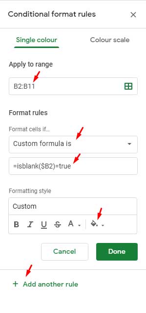
Click on the “Is not empty” drop-down and select “Custom formula is”. You will see a blank field. Copy-paste the above rule #1 in the blank field.
Under the field, you can see “Formatting style”. Click on the paint bucket similar icon (fill color) and select “None”.

Once complete, click “Add another rule” and enter rule # 2 in the custom formula field.
This time choose your preferred color (other than white/none) to highlight the max value and click “Done”.
Different Group Column and Value Column – How to Modify Formula Rules?
Suppose the group column is B instead of column A and the max value column is column E instead of column B. Here are the changes in the formula.
Modified Rule # 1:
=isblank($E2)=trueModified Rule # 2:
=isna(vlookup(B2&E2,ArrayFormula(index(sortn(sort({$B$2:$B,$E$2:$E},1,0,2,0),9^9,2,1,0),0,1)&index(sortn(sort({$B$2:$B,$E$2:$E},1,0,2,0),9^9,2,1,0),0,2)),1,0))=falseIn modified rules 1 and 2, the “Apply to range” in conditional format settings will change to E2:E11 from B2:B11.
How Rule # 2 Formula Highlights the Max Value in Each Group?
Below I am going to explain the key formula, which is rule # 2, step-by-step.
The SORT formula sorts the items and values in descending order. So the max value of each group will be on the top row of each group.
=sort({$A$2:$A,$B$2:$B},1,0,2,0)The SORTN removes the duplicates from the group and retains the top row in each group.
=sortn(sort({$A$2:$A,$B$2:$B},1,0,2,0),9^9,2,1,0)| Orange | 75 |
| Mango | 125 |
| Apple | 255 |
To understand this SORTN feature (removing duplicates from each group) you can read my post; SORTN Tie Modes in Google Sheets – The Four Tiebreakers.
Now we have the max values of each group and the corresponding max item names.
Using two Index formulas we can separate the columns (item names and the max values columns).
Extract Item Name (first column):
=index(sortn(sort({$A$2:$A,$B$2:$B},1,0,2,0),9^9,2,1,0),0,1)
Extract Max Values (second column):
=index(sortn(sort({$A$2:$A,$B$2:$B},1,0,2,0),9^9,2,1,0),0,2)
Then with the help of the & operator, combined the two columns (two Index formulas) as below.
Additionally, I have wrapped these Index formulas with ArrayFormula as the & operator used in an array.
=ArrayFormula(index(sortn(sort({$A$2:$A,$B$2:$B},1,0,2,0),9^9,2,1,0),0,1)&index(sortn(sort({$A$2:$A,$B$2:$B},1,0,2,0),9^9,2,1,0),0,2))| Orange75 |
| Mango125 |
| Apple255 |
The above values are the ‘range’ in a vertical lookup (Vlookup) which is our final formula that highlights the max value in each group in our Google Spreadsheet file.
Syntax:
VLOOKUP(search_key, range, index, [is_sorted])Now time to take a look at our data in A2:B11 and the Vlookup ‘search_key’ below.
=A2&B2This returns “Apple100” as the search_key. The ‘index’ (output column number in Vlookup) is 1 as there is only 1 column in the ‘range’.
Vlookup won’t find the above ‘search_key’ in the ‘range’ and so it would return FALSE.
Next, the Vlooup will use the search_key “Apple255” (A3&B3) in the ‘range’ and would return a TRUE.
Since the value is TRUE, the corresponding cell in the range B2:B11 will be highlighted. This continues down the row.
That’s all about highlighting the max value in each group in Google Sheets.
More Posts on Conditional Formatting
- Multiple OR in Conditional Formatting Using Regex in Google Sheets.
- Date Related Conditional Formatting Rules in Google Sheets.
- How to Conditional Format Duplicates Across Sheet Tabs in Google Sheets.
- Highlight an Entire Row in Conditional Formatting in Google Sheets.
- How to Highlight All Error Rows in Google Sheets.
- How to Highlight Largest 3 Values in Each Row in Google Sheets.
- Find All the Cells Having Conditional Formatting in Google Sheets.
- How to Highlight Cells Containing Specific Function in Google Sheets.
- Highlight Groups When Group Total Exceeds Target in Google Sheets.
- How to Highlight Vlookup Result Value in Google Sheets.
- Highlight Partial Matching Duplicates in Google Sheets.


Can you use this same technique to find the minimum in each group?
Hi, Randall Revere,
It’s so simple. Please check my new tutorial – How to Highlight the Min Value in Each Group in Google Sheets.
PERFECT!!! Thank you
Hi, Randall Revere,
I’ve modified the post. You can find a much simpler Rule # 2 there now.
Copy that instead.
=B1=MAX(FILTER(B:B, A:A=A1))Where;
A is the category column.
B is the value column.
Hi, Dev L,
This is cool! Thanks for sharing.