When analyzing data in Google Sheets, you may need to highlight groups when their total exceeds a target. This helps you quickly identify product categories, teams, or departments that surpass performance thresholds—using just a few formulas. In this tutorial, you’ll learn how to use conditional formatting to highlight groups when their total exceeds a target in Google Sheets.
We’ll primarily focus on a single-table format, where both the target and actual values are in the same table. We’ll also briefly cover how to work with separate target and actual tables using lookup functions.
Note: This tutorial is about highlighting entire groups when their total exceeds or meets a target. Each group can have the same target or its own individual target—stored either within the main table or in a separate lookup table.
If you’re instead looking to:
- Highlight each group based on a single shared target using a basic SUMIF condition (e.g., if a student’s total attendance meets 120 days), check out: How to Use SUMIF in Conditional Formatting in Google Sheets
- Highlight the specific rows involved in a SUMIFS calculation—and optionally apply a condition based on the total—see: Highlight SUMIFS Rows Based on Their Total in Google Sheets
Generic Formula to Highlight Groups When Their Total Exceeds a Target
=SUMIF(Group_Range, Current_Group, Value_Range) > Target_CellExplanation:
Group_Range: The column containing group names/items/categories. (e.g.,$A$2:$A)Current_Group: The specific group/item being evaluated. (e.g.,$A2)Value_Range: The column with actual values to sum. (e.g.,$C$2:$C)Target_Cell: The reference cell containing the target value. (e.g.,$B2)
Let’s apply this to sample data.
Step 1: Set Up the Sample Data
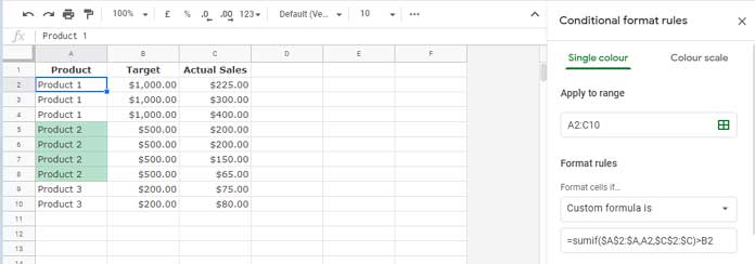
The sample data consists of products in column A, their target values in column B, and actual sales in column C.
Since column A is sorted by product, you can easily verify group totals and compare them against targets. Sorting is not required for the highlighting to work.
Note: In this setup, each group (e.g., product or category) has its target repeated in column B for every row that belongs to that group. This makes it easier to compare each group’s total using a simple SUMIF formula without needing a separate lookup.
Step 2: Apply Conditional Formatting to Highlight Groups When Their Total Exceeds the Target
Steps to Apply the Conditional Formatting Rule:
- Select the range → Select A2:A10 (or A2:C10 if you want to highlight all columns).
- Go to → Click Format > Conditional formatting.
- Choose Rule Type → Under Format rules, select Custom formula is.
- Enter the Formula →
=SUMIF($A$2:$A, $A2, $C$2:$C) > $B2 - Choose Formatting Style → Pick a highlight color.
- Click Done → The groups where the total exceeds the target will now be highlighted.
Highlight Groups When the Total Meets or Exceeds the Target
If you also want to highlight groups that meet or exceed the target, use this formula instead:
=AND(N($B2), SUMIF($A$2:$A, $A2, $C$2:$C) >= $B2)Handling Separate Target and Actual Tables
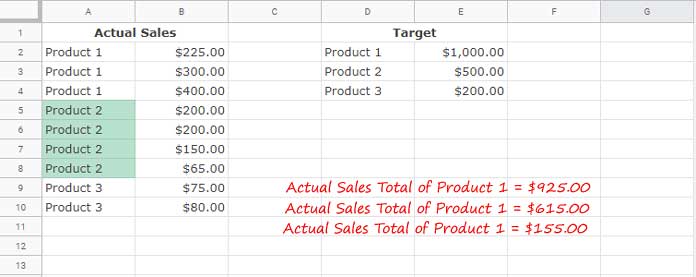
In the above example, the target and actual values are in the same table. However, sometimes targets are stored in a separate table. In that case, you can use XLOOKUP to fetch the target value corresponding to each group:
Generic Formula for Separate Target and Actual Tables
=SUMIF(Group_Range, Current_Group, Value_Range) > XLOOKUP(Current_Group, Target_Lookup_Range, Target_Value_Range)Explanation:
Group_Range: The column containing group names (e.g.,$A$2:$A).Current_Group: The specific group being evaluated (e.g.,$A2).Value_Range: The column with actual values to sum (e.g.,$B$2:$B).Target_Lookup_Range: The column in the target table containing group names (e.g.,$D$2:$D).Target_Value_Range: The column in the target table containing the target values (e.g.,$E$2:$E).
Example Formulas:
- Highlight when the total exceeds the target:
=SUMIF($A$2:$A, $A2, $B$2:$B) > XLOOKUP($A2, $D$2:$D, $E$2:$E) - Highlight when the total meets or exceeds the target:
=SUMIF($A$2:$A, $A2, $B$2:$B) >= XLOOKUP($A2, $D$2:$D, $E$2:$E)
Additional Tips & Wrap-up
Ensure the correct data range is selected before applying conditional formatting. If you’re using a separate target table, make sure the group names match exactly, avoiding extra spaces or inconsistent capitalization.
I recommend using XLOOKUP to fetch target values, but you can also use VLOOKUP.
By following this tutorial, you can highlight groups when their total exceeds a target in Google Sheets, making it easier to analyze data trends and spot key performance insights. Whether your target and actual values are in one table or separate tables, you can apply the right formula and formatting rule to get accurate results.
Let me know if you have any questions!
Conclusion
Highlighting groups based on whether their totals exceed a target helps you quickly identify high-performing categories without manual checks. Using SUMIF within conditional formatting keeps the setup simple, whether your targets are in the same table or fetched using lookup functions.
If you’d like to explore more conditional formatting techniques—from basic rules to advanced formula-driven methods—check out the Ultimate Guide to Conditional Formatting in Google Sheets, where all related tutorials are organized in one place.


