How to Highlight Entire Error Rows in Google Sheets

There is no built-in rule to highlight entire error rows in a range in Google Sheets. To achieve this, you need to use a custom formula.

This tutorial answers:

How to highlight an entire row if one of the cells in that row contains an error.
How to apply this to all rows in the range.

The errors can be any type, including #N/A, #DIV/0!, #REF!, and #VALUE!.

That’s exactly what we’ll cover in this tutorial.

Table of Contents

Example of Highlighting Entire Error Rows in Google Sheets

Assume you have the following sample data:

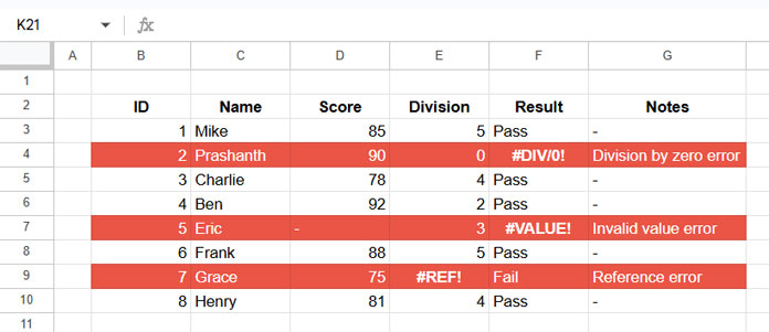
Google Sheets table with sample data, showing entire rows highlighted in red where errors like #N/A and #DIV/0! are present

You can use the following custom formula to highlight all error rows in the data, which in this example are rows 4, 7, and 9. The formula will highlight the entire row if any cell in that row contains an error.

=ArrayFormula(XMATCH(TRUE, ISERROR($B3:$G3)))

Steps to Apply the Formula:

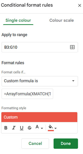
Select the range B3:G10.
Click Format > Conditional Formatting to open the Conditional format rules panel.
Under Format Rules, select Custom formula is.
Copy and paste the above formula.
Choose a fill color, such as red.
Click Done.

Google Sheets Conditional Formatting panel with custom formula rule applied to highlight entire rows containing errors

This will highlight all error rows in the selected range.

Adjusting the Formula for a Different Range

Your data range may not be the same as in the example. In that case, you can easily modify the formula.

For example, if your range is A1:Z1000, the formula would be:

=ArrayFormula(XMATCH(TRUE, ISERROR($A1:$Z1)))

In the Conditional format rules panel, set the Apply to range as A1:Z1000.

Breaking Down the Formula That Highlights Entire Error Rows in Google Sheets

The rule works as follows:

The ISERROR($B3:$G3) function checks for errors in each cell within the row and returns an array of TRUE and FALSE values.
The XMATCH(TRUE, ISERROR($B3:$G3)) function finds the first occurrence of TRUE (an error) in the row.
If an error is found, XMATCH returns its relative position within the array as a number, which is interpreted as TRUE in the conditional formatting rule, causing the entire row to be highlighted.
Since we use absolute column references ($B:$G) and relative row references, the rule applies to all rows in the selected range (B3:G10).

That’s how you can highlight entire error rows in Google Sheets.

Conclusion

This method helps you quickly identify error rows without manually scanning your data.

For more techniques, see The Ultimate Guide to Conditional Formatting in Google Sheets.