If you have many formulas spread across a sheet in Google Sheets, it’s easy to highlight all formula cells using the ISFORMULA function.

But what if you want to highlight only cells that contain a specific function — like VLOOKUP, SUMIF, or formulas using addition, subtraction, or division?

In this tutorial, I’ll show you exactly how to highlight specific functions or operators in Google Sheets using Conditional Formatting and REGEX formulas.

Highlight All Formula Cells in Google Sheets

Quick tip:

You can highlight all formula cells by using a custom formula with ISFORMULA.

Select the range A1:Z (or the entire sheet starting from A1). Then, in Format > Conditional formatting > Format rules > Custom formula, enter:

=ISFORMULA(A1)

This highlights all cells containing any formula.

But now let’s focus on highlighting only specific functions or operators.

How to Highlight Cells Containing a Specific Operator

Formulas often involve basic math operators like +, -, /, and *. We can highlight cells containing a certain operator by using the FORMULATEXT function with REGEXMATCH.

For example, suppose your sheet has addition formulas like:

• =A1+B1+C1
• =5+10+15

Here’s how to highlight only those cells:

Step 1: Select your range (e.g., A1:I5).

Click and drag to select the cells you want to apply the conditional formatting to. You can also click the first cell (A1), hold down Shift, and then click the last cell (I5) to quickly select the entire range.

Step 2: Use this custom formula in Conditional Formatting:

=REGEXMATCH(FORMULATEXT(A1), "\+")

This will highlight only cells containing the plus (+) operator.

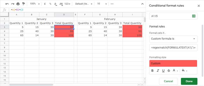
Why it Works

• FORMULATEXT(A1) converts the formula to text.
• REGEXMATCH looks for the + symbol inside the formula text.

Important:

If a cell doesn’t contain a formula (e.g., just text like “Mango+Orange”), FORMULATEXT returns #N/A, and such cells are ignored.

Highlight Cells with Subtraction, Division, or Multiple Operators

You can modify the regex to highlight different operators:

• Subtraction (-)
  =REGEXMATCH(FORMULATEXT(A1), "\-")
• Division (/)
  =REGEXMATCH(FORMULATEXT(A1), "\/")
• Both Addition and Subtraction
  =REGEXMATCH(FORMULATEXT(A1), "\-|\+")

This flexibility lets you target formulas using multiple operations!

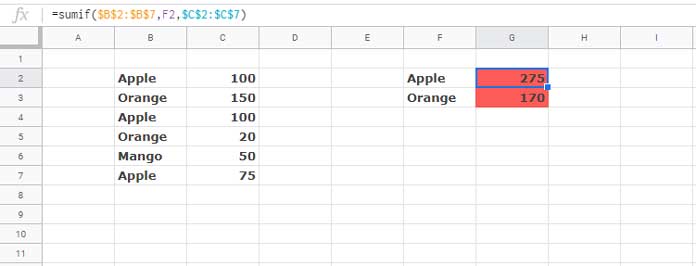
How to Highlight Cells Containing a Specific Function Like SUMIF or VLOOKUP

Suppose you want to highlight cells using the SUMIF function.

Here’s the Conditional Formatting formula:

=REGEXMATCH(FORMULATEXT(A1), "(?i)SUMIF")

• (?i) makes the match case-insensitive, so it works even if you type sumif, SUMIF, or SumIf.

Similarly, to highlight cells containing the VLOOKUP function:

=REGEXMATCH(FORMULATEXT(A1), "(?i)VLOOKUP")

Replace the function name in the formula (e.g., “SUMIF”, “VLOOKUP”) with any function you want to highlight.

Real-World Example Table

Apply the appropriate custom formula to highlight the matching cells!

Bonus Tip: Combine Multiple Functions

Want to highlight cells containing either SUMIF or VLOOKUP?

Use a regex that matches both:

=REGEXMATCH(FORMULATEXT(A1), "(?i)SUMIF|VLOOKUP")

This will highlight cells containing either function.

Conclusion

Using FORMULATEXT and REGEXMATCH, you can precisely highlight cells that contain a specific function or operator in Google Sheets.

Whether you want to catch SUMIF, VLOOKUP, addition, or subtraction formulas — you now know the exact steps to do it easily.

If you want to explore more conditional formatting techniques—such as lookups, duplicates, ranking, and advanced formula-based rules—check out: The Ultimate Guide to Conditional Formatting in Google Sheets

You May Also Like:

• How to Highlight Entire Error Rows in Google Sheets
• Google Sheets: Highlight an Entire Column If Any Cell Has an Error
• Highlight Invalid Entries in Drop-down Lists in Google Sheets
• Highlight Cells Containing Special Characters in Google Sheets