In this post, I aim to shed some light on making a case-insensitive regular expression match using the REGEXMATCH function in Google Sheets.
Additionally, you will learn how to make only part of a regular expression case-sensitive.
As far as I know, REGEXMATCH (RE2 expressions) and QUERY are the functions that use regular expressions, especially for text matching. This post is about the former.
Notes:
- In Google Sheets QUERY, we can use the MATCHES string comparison operator for a (preg) regular expression match.
- Two more functions in Google Sheets use RE2 regular expressions: REGEXREPLACE and REGEXEXTRACT. Besides matching, they perform additional tasks.
What Is Case Sensitivity in Text Matching?
It’s all about whether the text is sensitive or insensitive to the capitalization of letters.
In other words, whether uppercase and lowercase letters are treated as distinct or equivalent.
Please see the table below.
| Text 1 | Text 2 | Output (Sensitive to Capitalization) | Output (Insensitive to Capitalization) |
| Apple | APPLE | FALSE | TRUE |
| Orange | Orange | TRUE | TRUE |
| ORANGE | APPLE | FALSE | FALSE |
I want to match the values in column 1 with the values in column 2 in two different ways.
I have done this, and the outputs in columns 3 and 4 are self-explanatory.
Case-Insensitive REGEXMATCH in Google Sheets (Whole)
Let’s start with the basic formulas first (whole matching). We will later discuss how to make only part of a regular expression case-sensitive in Google Sheets.
With the Help of Text Functions LOWER or UPPER
We usually use the text functions LOWER, UPPER, or PROPER for case-insensitive regex matching in Google Sheets. The idea is to change the case of the text to be tested and match the same case in the pattern.
Assume you have entered the text abCDef in cell A1 and inserted the following REGEXMATCH formula in cell B1:
=REGEXMATCH(A1, "abcdef")It will return FALSE.
You can use the LOWER function as below for case-insensitive regex matching in Google Sheets:
=REGEXMATCH(LOWER(A1), "abcdef")If the regular_expression is a cell reference, for example, B1, you should use LOWER(B1), UPPER(B1), or PROPER(B1) depending on A1’s letter case:
=REGEXMATCH(UPPER(A1), UPPER(B1))With the Help of a Pattern Modifier
There is one drawback to using the LOWER/UPPER/PROPER text functions for case-insensitive regex matching in Google Sheets. What is it?
When using either of these two functions, we can’t make part of the REGEXMATCH regular expression case-sensitive.
In that scenario, the pattern modifier, i.e., (?i), does the job. We will come to that later.
First, learn about replacing the above ‘change case’ functions (UPPER/LOWER/PROPER) with the said pattern modifier.
This time, in B1, we can use the following formula:
=REGEXMATCH(A1, "(?i)abcdef")We can follow this method when using cell references in both arguments:
=REGEXMATCH(A1, "(?i)" & B1)Making Only Part of a Regular Expression Case-Sensitive in REGEXMATCH
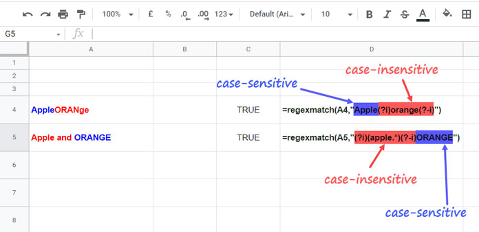
The sample text in cell A4 is AppleORANge. How do I make part of this text, i.e., Apple, case-sensitive, and the other part, i.e., ORANge, case-insensitive?
You can use this formula in C4.
=REGEXMATCH(A4, "Apple(?i)orange(?-i)")The text in cell A5 is Apple and ORANGE. To make the first part case-insensitive and the second part case-sensitive, use the following formula in cell C5:
=REGEXMATCH(A5, "(?i)(apple.*)(?-i)ORANGE")The .* part matches any character zero or more times.
That’s all about case-insensitive REGEXMATCH in Google Sheets. You can find some related resources below.


