In Google Sheets, we can use a regex function (which uses RE2 regular expressions) to get all words after the nth word in a sentence. This is especially useful when you want to extract specific parts of text consistently.

The most suitable function for this task is REGEXREPLACE. Another approach involves a combination of INDEX, SPLIT, and SUBSTITUTE, which we will also explore.

Note: We use REGEXREPLACE, not REGEXEXTRACT, because we want to remove the first n words and retain the rest of the sentence.

Get All Words after Nth Word Without Using Regex in Google Sheets

Suppose you have product details following a country code, item number, and batch number in a string. You may want to remove the first three words to get just the clean product information.

For example, consider the following text in cell A1:

US 4589 BATCH23 Premium Quality Cotton Shirts for Men

To get all words after the third word, you can use this formula:

=INDEX(SPLIT(SUBSTITUTE(A1, " ", "🐠", 3), "🐠"), 0, 2)

Result:

Premium Quality Cotton Shirts for Men

Tip: Replace the number 3 with any other number to get all words after that nth word. For example, 5 would return all words after the fifth word.

How This Formula Works

1. SUBSTITUTE(A1, " ", "🐠", 3) – replaces the third space with a unique delimiter (🐠).
2. SPLIT(..., "🐠") – splits the text into two parts based on that delimiter.
3. INDEX(..., 0, 2) – returns the second column (everything after the nth word).

Applying the Formula to Multiple Rows (Array Formula)

The non-regex formula also works with ranges:

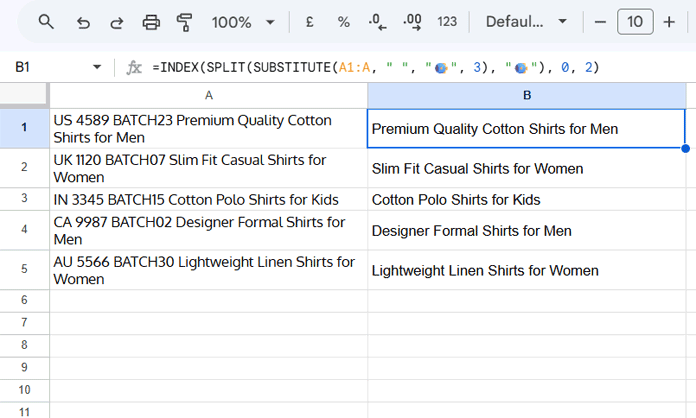
=INDEX(SPLIT(SUBSTITUTE(A1:A, " ", "🐠", 3), "🐠"), 0, 2)

Here, A1:A allows the formula to handle multiple cells at once.

Using Regex to Get All Words after Nth Word in Google Sheets

Using a regular expression simplifies the process, especially for dynamic nth-word extraction.

Understanding the Regular Expression

^(\S+\s+){3}

Explanation:

• ^ → anchors at the start of the string
• \S+ → matches one or more non-space characters (a whole word, including digits or symbols)
• \s+ → matches the following space(s)
• {3} → repeats 3 times (skip the first 3 words)

Replace with "" in REGEXREPLACE to remove the first n words.

For reference, see RE2 syntax on GitHub.

How to Use the Regex Formula in Google Sheets

=REGEXREPLACE(A1, "^(\S+\s+){3}", "")

This formula removes the first 3 words and returns the rest of the sentence.

Applying the Regex Formula to Multiple Rows (Array Formula)

The regex-based approach also works with ranges:

=ARRAYFORMULA(REGEXREPLACE(A1:A, "^(\S+\s+){3}", ""))

Conclusion

Using Regex to Get All Words after Nth Word in Google Sheets makes text extraction easy and flexible, whether for a single cell or an entire column. You can choose between the non-regex approach using INDEX, SPLIT, SUBSTITUTE, or the regex approach using REGEXREPLACE, depending on your preference and complexity of data.

Related Resources

• Extract, Replace, Match Nth Occurrence of a String or Number in Google Sheets
• Extract Every Nth Line from Multi-Line Cells in Google Sheets
• How to Match or Extract the Nth Word in a Line in Google Sheets
• Substitute the Nth Delimiter from Right in Google Sheets
• How to Replace Every Nth Delimiter in Google Sheets