The REGEXMATCH function is one of the popular text functions in Google Sheets. When inputting numbers, dates, or time values into any of the Regex text functions, you must adjust the formula accordingly. In this Google Sheets tutorial on how to use REGEXMATCH to match dates, I aim to provide clarification.

The REGEXMATCH function takes two arguments: text and regular_expression.

REGEXMATCH(text, regular_expression)

For both of these arguments, the function requires pure text values as input. Failure to provide text values will result in a VALUE! error, indicating that parameter 1 or parameter 2 values cannot be coerced into text.

You May Like:- Different Error Types in Google Sheets and How to Correct It.

Therefore, when attempting to use REGEXMATCH to match dates in Google Sheets, it is essential to convert them to plain text.

Regex Error in Date Column in Google Sheets

I have a date column as shown below in my dataset; Column A represents that date column. I aim to test whether a date in cell D2 or several dates in the range D2:D range are available or match in this date column.

Here’s my sample date column and the dates to match:

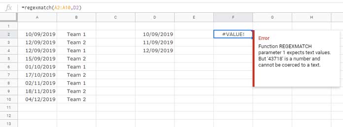
=REGEXMATCH(A2:A10, D2)

In cell F2, I attempted to use the above REGEXMATCH formula to check whether the date 10/09/2018 in cell D2 is present in the range A2:A10. However, the formula outputted an error value.

The above approach is not the correct way to use REGEXMATCH for dates in Google Sheets.

Below, you can find the correct details for matching a single date and multiple dates using the REGEXMATCH function in Sheets.

REGEXMATCH Formula to Match a Single Date in Google Sheets

To work with dates in REGEXMATCH, REGEXREPLACE, and REGEXEXTRACT functions in Google Sheets, it is necessary to convert the dates to plain text.

The TO_TEXT function facilitates the conversion of dates into plain text that can be used in regex operations. Therefore, the correct formula for using REGEXMATCH with a single date would be as follows:

=ArrayFormula(REGEXMATCH(TO_TEXT(A2:A10), TO_TEXT(D2)))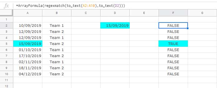

Note:

If the date formatting differs between column A and column D, meaning all dates are not formatted uniformly, the formula may not produce accurate matches.

To address this, you can either include the TEXT function to format the dates as illustrated below, or manually select the dates and navigate to Format > Number > Custom Date and Time, choosing an appropriate date format.

=ArrayFormula(REGEXMATCH(TO_TEXT(TEXT(A2:A10, "DD/MM/YYYY")), TO_TEXT(TEXT(D2, "DD/MM/YYYY"))))

TO_TEXT in a Date Range (Array) – Points to Note

You can observe the utilization of ArrayFormula in conjunction with TO_TEXT in the aforementioned Regex. Why is this necessary?

The sole parameter in the TO_TEXT function above is an array (date range). However, the TO_TEXT function itself is not designed as an array function. Therefore, when you input an array into TO_TEXT, it is essential to use ArrayFormula along with it.

Note:

If you opt to use the date regular_expression directly in the Regex, the following formula will work.

=ArrayFormula(REGEXMATCH(TO_TEXT(A2:A10), "15/09/2019")) // without text formatting
=ArrayFormula(REGEXMATCH(TO_TEXT(TEXT(A2:A10, "DD/MM/YYYY")), "15/09/2019")) // with text formatting

Match Multiple Dates or Date Range Using Regex Formula in Google Sheets

As mentioned earlier, it is imperative to include the TO_TEXT and ArrayFormula functions in this context as well.

The distinction lies in amalgamating multiple dates to form the required regular expression. Still confused?

To use REGEXMATCH with multiple dates in Google Sheets, employ the formula below. Each date to match should be separated by a pipe symbol.

=ArrayFormula(REGEXMATCH(TO_TEXT(A2:A10), "15/09/2019|17/10/2019|02/11/2019"))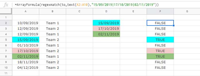

Note: Include the TEXT function if it is deemed necessary, as demonstrated in our earlier examples above.

Wondering how to incorporate the dates in D2:D4 instead of using the text “15/09/2019|17/10/2019|02/11/2019” as the regular expression.

The following TEXTJOIN function combines the dates in D2:D4 according to the aforementioned regular expression pattern.

=TEXTJOIN("|", TRUE, D2:D4)

Applying the above guidance, the REGEXMATCH formula to match multiple dates is as follows:

=ArrayFormula(REGEXMATCH(TO_TEXT(A2:A10), TEXTJOIN("|", TRUE, D2:D4)))

Note: The subsequent section contains additional tips. You may choose to skip it or continue reading.

Regex to Filter Matching Multiple Dates in Google Sheets

All the formulas provided above for Regexmatch dates yield Boolean TRUE and FALSE values as the output.

To filter multiple matching dates, you can utilize these Boolean values (i.e., the Regexmatch formula itself) as the filter criteria:

=FILTER(A2:B10, ARRAYFORMULA(REGEXMATCH(TO_TEXT(A2:A10), TEXTJOIN("|", TRUE, D2:D4))))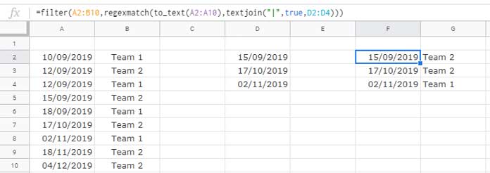

Please note that the inclusion of ArrayFormula around the Regex is not mandatory within the FILTER function. You can alternatively use the Filter formula without it, as shown below:

=FILTER(A2:B10, REGEXMATCH(TO_TEXT(A2:A10), TEXTJOIN("|", TRUE, D2:D4)))

That concludes the discussion on Regexmatch Dates in Google Sheets. Thank you for your attention. Enjoy!

Additional Resources:

1. REGEXMATCH in SUMIFS and Multiple Criteria Columns in Google Sheets.
2. Match Two Columns that Contain Values Not in Any Order Using Regex.
3. Multiple OR in Conditional Formatting Using Regex in Google Sheets.
4. Matches Regular Expression Match in Google Sheets Query.
5. Highlight Matches or Differences in Two Lists in Google Sheets.