When you want to match values in two columns in any order, you can use various approaches in Google Sheets. One effective option is using REGEXMATCH. The advantage of REGEXMATCH is its flexibility, allowing you to perform case-sensitive or case-insensitive matches.

Example:

=ArrayFormula(
   IF(
      A2:A="",,
      REGEXMATCH(A2:A, "(?i)^"&TEXTJOIN("$|^", TRUE, UNIQUE(B2:B))&"$"))
)

This formula matches the values in columns A and B, returning TRUE wherever a match is found in the same row or any row in the range, and FALSE otherwise.

Note: This is a text function and works only with text values. If the columns contain numeric values, use XMATCH instead. Alternatively, you can format numeric values as text and apply REGEXMATCH, but this may lead to issues such as 10.2 not matching 10.20.

Matching Numeric Columns

For numeric values, use the following XMATCH formula:

=ArrayFormula(
   IF(
      A2:A="",,
      XMATCH(A2:A, B2:B)
   )
)

This matches numeric values in column A with those in column B, effectively matching values between two columns in any order.

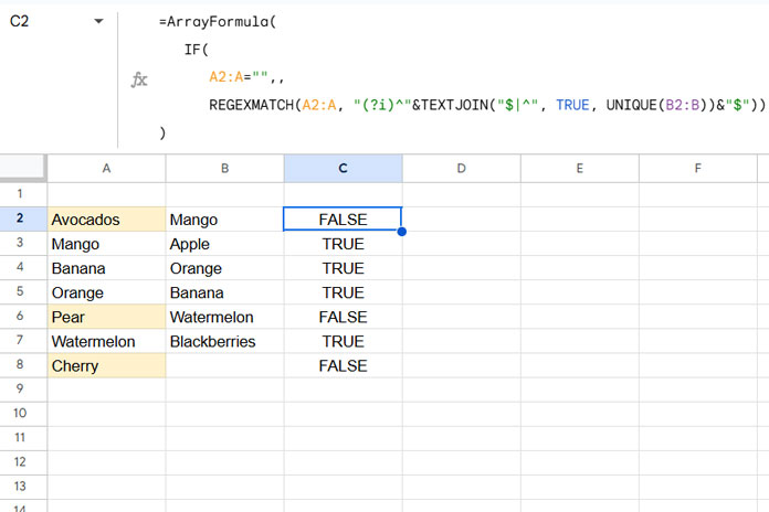
Example: Matching Two Text Columns with Values in Any Order

Assume you have item names in columns A and B that are unordered. Use the following formula in cell C2:

=ArrayFormula(
   IF(
      A2:A="",,
      REGEXMATCH(A2:A, "(?i)^"&TEXTJOIN("$|^", TRUE, UNIQUE(B2:B))&"$"))
)

This formula returns TRUE for rows where the value in column A has a match in column B, and FALSE otherwise. Items with FALSE are not present in column B.

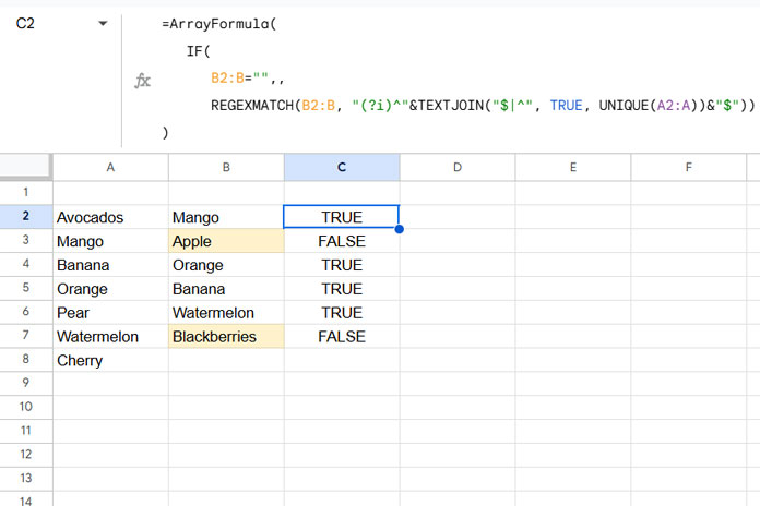
To check items in column B that are not in column A, use:

=ArrayFormula(
   IF(
      B2:B="",,
      REGEXMATCH(B2:B, "(?i)^"&TEXTJOIN("$|^", TRUE, UNIQUE(A2:A))&"$")
   )
)

To perform a case-sensitive match, remove (?i) from the formulas.

Example: Matching Two Numeric Columns with Values in Any Order

For numbers or dates in unordered columns, use the following XMATCH formula instead of REGEXMATCH, as REGEXMATCH is designed for text fields:

=ArrayFormula(
   IF(
      A2:A="",,
      IFNA(XMATCH(A2:A, B2:B))
   )
)

The formula returns a blank for items in column A that it does not find in column B. To check items in column B that are not in column A, use:

=ArrayFormula(
   IF(
      B2:B="",,
      IFNA(XMATCH(B2:B, A2:A))
   )
)

Note: These formulas work for text columns as well, but unlike REGEXMATCH, XMATCH is not case-sensitive.

Additional Tips: Filtering

You can use the above formulas as filter conditions. Here is the syntax for the FILTER function:

FILTER(range, condition1, [condition2, …])

Example: Filtering Column A for Items Not in Column B

=FILTER(A2:A, NOT(IF(A2:A="",,REGEXMATCH(A2:A, "(?i)^"&TEXTJOIN("$|^", TRUE, UNIQUE(B2:B))&"$"))))

This extracts values from column A that are not present in column B.

Similarly, to filter column B for values not in column A:

=FILTER(B2:B, NOT(IF(B2:B="",,REGEXMATCH(B2:B, "(?i)^"&TEXTJOIN("$|^", TRUE, UNIQUE(A2:A))&"$"))))

You can replace the condition with XMATCH as well.

Resources

• How to Compare Two Columns for Matching Values in Google Sheets
• How to Match Multiple Values in a Column in Google Sheets
• How to Perform Partial Match Between Two Columns in Google Sheets
• REGEXMATCH in FILTER Criteria in Google Sheets [Examples]
• Case-Insensitive REGEXMATCH in Google Sheets (Partial or Whole)
• NOT in REGEXMATCH and Alternatives in Google Sheets