You can use the FILTER function with COUNTIF or ISNA+MATCH to compare two lists and extract the differences in Google Sheets.
You can compare List 1 with List 2 to extract the items in List 1 that are not available in List 2 and vice versa.
For example, I have received a quotation from a vendor for plumbing materials. Their quotation is based on the availability of materials with them. Now, I can compare this list with my requirements in two different ways:
- I can compare the list provided by the vendor with my original requirements and find the unavailable items.
- I can also find the items in the vendor’s list that do not match my requirements.
Compare Two Lists and Extract Differences: Understanding the Scenario
My requirements are listed in column A (A2:A), and what the vendor offered (quoted) is listed in column B (B2:B).
| Requirement | Offered by Vendor | Items Not Available with the Vendor | Additional Items Offered |
| Copper Pipes | UPVC Pipes | Copper Pipes | Health Faucets |
| UPVC Pipes | Health Faucets | Brass Fittings | Water Heaters |
| Brass Fittings | Shower Heads | Drain Pipes | Concealed Valve |
| Drain Pipes | Water Heaters | ||
| Shower Heads | Water Filters | ||
| Water Filters | Concealed Valve |
Since it’s a small list, you can manually find the items that are not in the offered list, but it’s not feasible for larger requirements. This is where formulas become helpful.
With the help of a custom Google Sheets formula, I’ve found those items in column C (C2:C).
In column D, I have listed the additional items that the vendor offered (quoted), which are not in my original requirements in column A.
In Google Sheets, you can easily compare two lists and extract the differences as shown above.
Compare Column A with Column B and Extract Non-Present Items
This is useful for finding items you want but are unavailable from the vendor. Your items are in column A, and the items available from the vendor are in column B.
As mentioned, you can use either FILTER with COUNTIF or FILTER with ISNA+MATCH. Here are both solutions:
You can try the following formulas in cell C2:
Solution 1:
=FILTER(A2:A, ISNA(MATCH(A2:A, B2:B, 0)))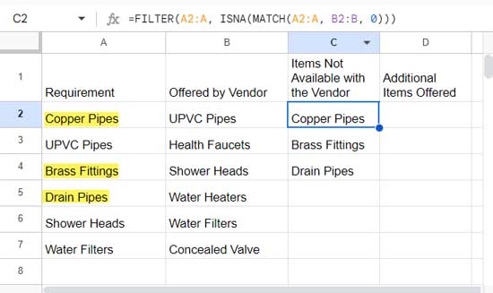
The FILTER function filters A2:A based on the condition ISNA(MATCH(A2:A, B2:B, 0)).
What does this condition mean?
The MATCH function searches for the values in A2:A within B2:B and returns the relative positions of matching items or #N/A for items not found. ISNA returns TRUE for #N/A and FALSE for relative positions (matches).
The FILTER function filters rows where the condition is TRUE.
Solution 2:
=FILTER(A2:A, COUNTIF(B2:B, A2:A)=0)Here, the condition is COUNTIF(B2:B, A2:A)=0.
The COUNTIF function counts how many times each value in A2:A appears in B2:B. If it returns 0, it means that the value is not present in B2:B.
This allows you to compare two lists and extract the differences, or in other words, the non-matching items in List 1.
Compare Column B with Column A and Extract Non-Present Items
To compare column B values with column A values and extract the differences in column B, you can use the formulas above by swapping the ranges. These are useful for identifying items offered by the vendor that are not in your list.
Solution 1:
=FILTER(B2:B, ISNA(MATCH(B2:B, A2:A, 0)))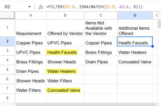
Solution 2:
=FILTER(B2:B, COUNTIF(A2:A, B2:B)=0)Here, the FILTER formula filters B2:B based on the given conditions.
This way, we can compare two lists and extract the differences in Google Sheets.
Resources
- Compare Two Sets of Multi-Column Data for Differences in Google Sheets
- How to Compare Two Sheets in Google Sheets for Mismatch
- Anti-Join in Google Sheets: Find Unmatched Records Easily
- How to Compare Two Columns for Matching Values in Google Sheets
- Compare Two Rows and Find Matches in Google Sheets
- Compare All Columns with Each Other for Duplicates in Google Sheets


Hey, Thank you.
What if the item repeats?
Say, for example, Item 6 is twice in column A and only once in column B.
Hi, Mithun P R,
In the formula, replace the first occurrence of A2:A with
A2:A&COUNTIFS(row(A2:A),"<="&row(A2:A),A2:A,A2:A)Similarly replace B2:B with
B2:B&COUNTIFS(row(A2:A),"<="&row(A2:A),B2:B,B2:B)Formula in C2:
=ArrayFormula(sort(if(COUNTIF(B2:B&COUNTIFS(row(A2:A),"<="&row(A2:A),B2:B,B2:B),A2:A&COUNTIFS(row(A2:A),"<="&row(A2:A),A2:A,A2:A))=0,A2:A,)))I have actually added a running count of A2:A values to make them unique.
You may also like this - Make Duplicates to Unique by Assigning Extra Characters in Google Sheets.
Great article, helped me a lot!
But although I could do what I intended in my project, I still don’t understand one thing. Could you explain this or direct me to some reading that does?
In the formula:
=sort(if(COUNTIF(A2:A,B2:B)=0,B2:B,))The IF returns blank if there is a difference and it is false, doesn’t it?
Then the SORT returns the list of values that are different. I don’t understand how the SORT function gets these values or what the IF is actually returning as value_if_false.
Hi, gustavo,
To understand the logic, please make a table as per my example (cell range A1:B7).
Then in cell H2, insert the below Countif.
=ArrayFormula(COUNTIF(A2:A10,B2:B10))Note:- You won’t see ArrayFormula use in my original formula. I’ll come to that below.
You can see that it returns the numbers 1 and 0 (against B2:B10). The number 1 for the match and 0 for the mismatch.
The logical_expression in IF is
ArrayFormula(COUNTIF(A2:A10,B2:B10))=0value_if_true – return values from B2:B10
value_if_flase – return blank
The SORT plays two roles.
1. It’s an alternative to the above ArrayFormula use. So COUNTIF works without any issue in a cell range.
2. The second one is most important. Without SORT, you may have blanks between the values in the IF result. By sorting, we can solve it.
This is a great help, thanks for the info. Could you help with how to get the count of the number of items in column A which are not present in Column B?
=counta(A2:A)-sum(ArrayFormula(countif(A2:A,B2:B)))