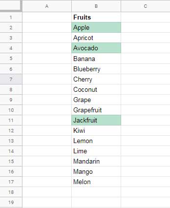
Assume you have a column with several keywords and want to highlight multiple values using a single rule. When applying multiple OR conditions in conditional formatting in Google Sheets, one of the most efficient approaches is to use the REGEXMATCH function.

Of course, you can also use the OR function. It works well, but as your criteria grow, REGEXMATCH becomes more scalable and easier to maintain.

Other alternatives include functions like MATCH, XMATCH, SEARCH, and FIND, which we’ll also cover later.

Why Use REGEXMATCH for Multiple OR Conditions?

Using REGEXMATCH offers several advantages:

• Easier to scale with many conditions
• Cleaner and more compact formulas
• Supports partial matching
• Supports case-sensitive and case-insensitive matching

Using the OR Function to Highlight Multiple Keywords

Formula:

=OR(B2="Apple", B2="Avocado", B2="Jackfruit")

Use this in a conditional formatting rule applied to B2:B.

See also: AND, OR, and NOT in Conditional Formatting in Google Sheets

This is simple and readable, but becomes messy when the list grows.

Using REGEXMATCH for Multiple OR Conditions

While the OR function works well for a few conditions, it quickly becomes hard to manage as the list grows. This is where REGEXMATCH offers a more scalable and cleaner alternative.

Formula:

=REGEXMATCH(B2,"Apple|Avocado|Jackfruit")

Just separate conditions using the pipe (|) symbol.

Common Issues and Fixes

Issue #1: Partial Matches

By default, REGEXMATCH performs partial matching.

Example:

=REGEXMATCH(B2,"Apple|Mango")

This matches:

• Apple
• Apple – Brazil

Fix: Use Anchors for Exact Match

=REGEXMATCH(B2,"^Apple$|^Mango$")

Issue #2: Case Sensitivity

Regex is case-sensitive by default.

Fix: Use (?i) for Case-Insensitive Match

=REGEXMATCH(B2,"(?i)Apple|Mango")

Exact + Case-Insensitive:

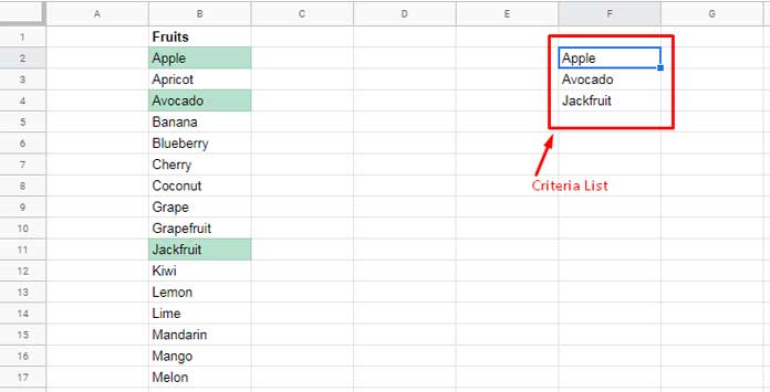
=REGEXMATCH(B2,"(?i)^Apple$|^Mango$")

Using a Criteria List (Best Practice)

So far, we’ve hardcoded the conditions. In practice, it’s more efficient to store them in a range (e.g., F2:F) and reference that list.

Partial Match (Case-Sensitive)

=REGEXMATCH(B2, TEXTJOIN("|", TRUE, $F$2:$F))

Exact Match (Case-Sensitive)

=REGEXMATCH(B2, "^"&TEXTJOIN("$|^", TRUE, $F$2:$F)&"$")

Exact Match (Case-Insensitive)

=REGEXMATCH(B2, "(?i)^"&TEXTJOIN("$|^", TRUE, $F$2:$F)&"$")

This is the most scalable approach for real-world datasets.

Alternative Methods

While REGEXMATCH is the most flexible approach, it’s not the only option. Depending on your use case, other functions may be more suitable.

MATCH / XMATCH

Hardcoded:

=MATCH(B2, TOCOL({"Apple","Avocado","Jackfruit"}), 0)

From Range:

=MATCH(B2, TOCOL($F$2:$F,1), 0)

You can replace MATCH with XMATCH for more flexibility.

SEARCH / FIND (Not Recommended)

These are less clean and mainly useful for partial matches.

=ARRAYFORMULA(SUM(IFERROR(SEARCH(TOCOL({"Apple","Avocado","Jackfruit"}),B2))))

• SEARCH → case-insensitive
• FIND → case-sensitive

Conclusion

When working with multiple OR conditions in conditional formatting in Google Sheets, REGEXMATCH stands out as the most flexible and scalable solution—especially when combined with TEXTJOIN for dynamic criteria lists.

While functions like OR, MATCH, or SEARCH can handle simpler scenarios, regex-based rules provide better control over exact vs partial matches and case sensitivity, making them ideal for real-world datasets.

If you want to explore more techniques like this—from basic rules to advanced formula-driven conditional formatting—refer to the hub:
The Ultimate Guide to Conditional Formatting in Google Sheets