Highlight Partial Matching Duplicates in Google Sheets

Quick Answer:
To highlight partial matching duplicates in Google Sheets, use this custom formula in conditional formatting:

=ArrayFormula(
   LET(
      range, $B$2:$B$15, 
      cell, B2, 
      test1, COUNT(IFERROR(SEARCH(cell, range))), 
      test2, COUNT(IFERROR(SEARCH(IF(range="", NA(), range), cell))), 
      test3, cell<>"", 
      AND(OR(test1>1, test2>1), test3)
   )
)

Table of Contents

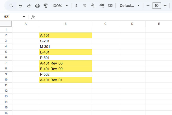
What Are Partial Matching Duplicates?

Partial matching duplicates occur when one value fully or partially exists within another value.

Example:

A-101
A-101 Rev. 00
A-101 Rev. 01

All of the above should be treated as duplicates because they share the same base value.

However, Google Sheets does not provide a built-in rule to highlight such matches—only exact duplicates.

Why Simple Formulas Fail

A common attempt is:

=AND(B2<>"", COUNTIF($B$2:$B$15, "*"&B2&"*")>1)

Problem:

Only highlights base values (e.g., A-101)
Fails to highlight revisions (A-101 Rev. 00)
Can produce false matches in mixed text datasets

Best Formula to Highlight Partial Matching Duplicates

Use this formula:

=ArrayFormula(
   LET(
      range, $B$2:$B$15, 
      cell, B2, 
      test1, COUNT(IFERROR(SEARCH(cell, range))), 
      test2, COUNT(IFERROR(SEARCH(IF(range="", NA(), range), cell))), 
      test3, cell<>"", 
      AND(OR(test1>1, test2>1), test3)
   )
)

Example showing partial matching duplicates highlighted in Google Sheets

Why This Works

Matches both directions:
- cell inside range
- range inside cell
Avoids false positives from blanks
Highlights all related entries, not just the first

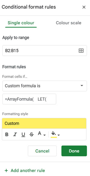
How to Apply the Rule

Select your data range (e.g., B2:B15)
Go to Format > Conditional formatting
Choose Custom formula is
Enter the formula above
Choose a formatting style
Click Done

Custom rule settings for partial matches in the Conditional Format panel in Google Sheets

How the Formula Works (Simple Explanation)

The formula uses three logical checks:

Search current cell in the range → finds larger matches
Search range values inside current cell → finds base matches
Ignore blank cells

If either match count is greater than 1, the value is considered a duplicate.

Important Note (Avoid False Positives)

Consider these values:

A-101 – Architectural Floor Plan (Level 1)
A-101 – Architectural Floor Plan (Level 2)

These are not true duplicates, even though they look similar.

But these are duplicates:

A-101
A-101 – Architectural Floor Plan (Level 2)

👉 If your data includes structured text, consider:

splitting columns
or extracting base values using LEFT or REGEXEXTRACT

When to Use This Method

Use this approach when:

You have codes with revisions
Data contains partial overlaps
Exact duplicate rules are not sufficient

Conclusion

This tutorial is part of The Ultimate Guide to Conditional Formatting in Google Sheets, where you can explore 80+ practical examples, including advanced duplicate detection, custom rules, and real-world use cases.

If you frequently work with versioned data or mixed text values, mastering partial match highlighting can significantly improve data analysis and cleanup.