Unlike Google Sheets REGEX text functions, LEFT, RIGHT functions are very straightforward to use. So little to learn the use of it. Further, you can replace both LEFT, RIGHT functions with REGEXEXTRACT.

First, I’m moving to the syntax part of the LEFT, RIGHT functions and then directly jumping to the alternative REGEXEXTRACT formula.

Google Sheets LEFT Function – Syntax

We can use Google Sheets LEFT function to return a specific number of characters from the left side of a String.

Syntax:

LEFT(string, [number_of_characters])

The below LEFT formula would return “INFO” the first four characters of the string.

=LEFT("INFO INSPIRED",4)

Google Sheets RIGHT Function – Syntax

The RIGHT function returns a specific number of characters from the right side of a specified string.

Syntax:

RIGHT(string, [number_of_characters])

The below RIGHT formula would return “INSPIRED” the last eight characters of the string.

=RIGHT("INFO INSPIRED",8)

See how we can replace or avoid LEFT, RIGHT functions with other functions in Google Sheets.

MID Function as an Alternative to LEFT, RIGHT functions in Google Sheets

You can use MID text function as an alternative to Google Sheets LEFT as well as RIGHT functions. Here is the example.

The below MID formula would return the word “INFO” which is equal to the above LEFT formula.

=MID("INFO INSPIRED",1,4)

The following MID formula would return the word “INSPIRED” similar to the above RIGHT formula.

=MID("INFO INSPIRED",6,8)

Now more interesting part of this tutorial. You can simply use REGEXEXTRACT as an alternative to Google Sheets LEFT as well as RIGHT functions.

See How REGEXEXTRACT Replaces LEFT, RIGHT Functions.

The following REGEXEXTRACT formula is equal to the LEFT formula above. It returns the first four characters from the string “INFO INSPIRED”

=REGEXEXTRACT("INFO INSPIRED","....")

Now you can similarly use REGEXEXTRACT to replace RIGHT function. The below formula would return the last 8 characters from the string.

=REGEXEXTRACT("INFO INSPIRED","(........\z)")

Practical Use of LEFT, RIGHT Functions

I am limiting this part to only one example as an effort to cut short this tutorial.

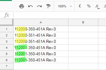
Let’s check how to find unique texts in a list when first few characters are only matching. Didn’t get? See the screenshot.

The above are few drawing numbers. I want to find the unique drawings based on the first 6 characters.

=ArrayFormula(countunique(left(A1:A6,6)))

See the formula. Here I’ve used the LEFT function in conjunction with COUNTUNIQUE and it would return the result as # 2.