Return Blank Instead of 30-12-1899 in Google Sheets Formulas

Did you notice that some of the Google Sheets formulas return 30-12-1899 when a date column is empty? How to return blank instead of 30-12-1899 in Google Sheets. Is there a quick solution to this?

There are a few good options to solve this puzzle, but that depends on the formula in use. For the example purpose, I am taking the functions MIN and MINIFS.

If you want solutions to formulas that involve some other functions, I mean to return blank instead of the default value of 30-12-1899, you can suggest the same in the comment section at the bottom of this page.

Update: A common solution to this problem was recently made available using the LET function. I’ve included that in the last part of this tutorial.

Why Do Some Google Sheets Formulas Return 30-12-1899?

In a formula, if you use a range of cells that contain dates and in which some of the cells are blank or 0, Google Sheets will treat those blank or 0 values as dates formatted to numbers.

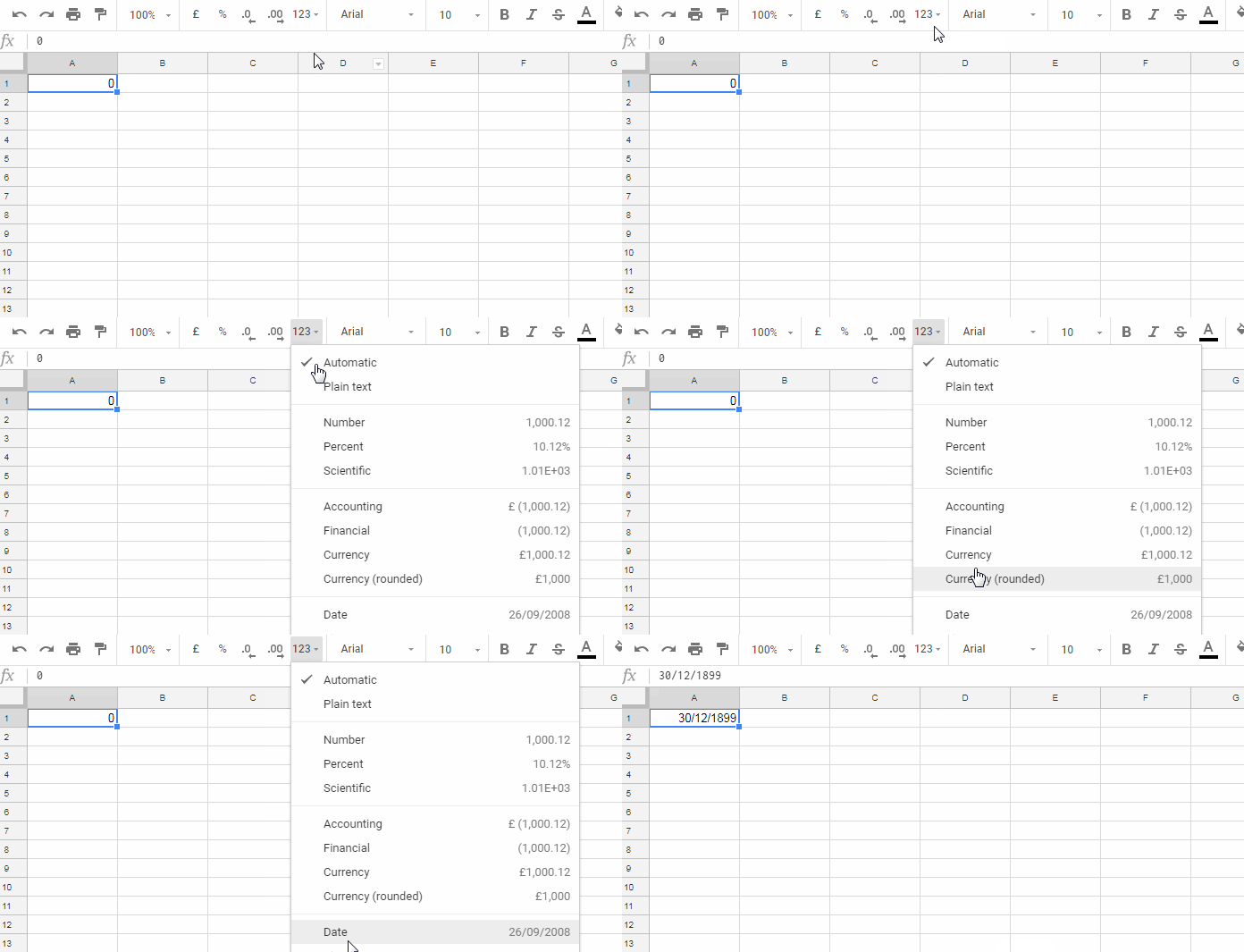
I can explain this better. If you format the number 0 as a date from the Format > Number > Date menu, you will get the date December 31, 1899.

Example showing why 0 becomes December 30, 1899 in Google Sheets

Change the number 0 to 1, and the date will become December 31, 1899.

If you format the number -1 as a date using the same steps, you will get the date December 29, 1899.

This is because Google Sheets stores dates as serial numbers so that they can be used in calculations. In Google Sheets, December 31, 1899 is serial number 1. Most functions automatically convert date values to serial numbers.

As a side note, Excel and Google Sheets use different date systems. The serial number 1 in Excel refers to January 1, 1900.

There are two possible scenarios where some of the formulas in Google Sheets return the date December 30, 1899:

When a formula returns a blank cell instead of a date.
When a formula returns the value 0 instead of a date.

In both cases, Google Sheets will treat the blank or 0 value as the date December 30, 1899.

Below are a few formula examples to help you learn how to return blank instead of 30-12-1899 in Google Sheets.

How to Return Blank Instead of 30-12-1899 in Google Sheets

We can filter out blanks or zeros from the source data to find a solution. However, if we do this, the “invalid” date will not appear, but some functions will not work and may return an “Argument must be a range” error. Therefore, we will tweak the formula output to return zero or blank instead of the “invalid” date if the formula output is 30-12-1899.

Example 1: Return Blank Instead of 30/12/1899 in MIN Function

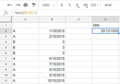
In a date range, I want to find the earliest date. The following MIN formula returns the date 30/12/1899 because there are cells with the value 0:

=MIN(B2:B11)

Return Blank Instead of 30-12-1899 in MIN Function

Here are two solutions:

Use the TEXT function to format the output to blank. This has a drawback: when there are no 0 values in the range, the returned date will be in text format.

=TEXT(MIN(B2:B11),"DD/MM/YYYY;;")

Use the SORTN function to return 0 instead of blank. Unlike MIN, the SORTN function will return 0 if the cells are blank or zero.

=SORTN(B2:B11)

Example 2: Formula to Return Blank Instead of 30/12/1899 in MINIFS Function

Unlike MIN, if the cells are blank or zero, functions like MINIFS, MAX, and MAXIFS usually return 0.

However, MINIFS and MAXIFS usually return date values, not formatted dates. As a result, we need to either apply the result cell with Format > Number > Date or use the TO_DATE function with the formula itself.

This causes the 30/12/1899 date issue when the result is 0. The MINIFS and MAXIFS results can be 0 when the criteria don’t match.

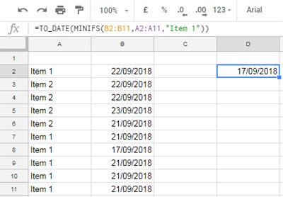
In the following example, we have item names in A2:A11 and purchase dates in B2:B11. The following MINIFS formula returns the earliest purchase date of “Item 1” in the range:

=TO_DATE(MINIFS(B2:B11,A2:A11,"Item 1"))

Return Blank Instead of 30-12-1899 in MINIFS Function

If we replace the criterion in the formula with “Item 3”, the formula will return 30/12/1899.

As an alternative to MINIFS, we can use the following FILTER + SORTN combination:

=SORTN(TO_DATE(IFNA(FILTER(B2:B11,A2:A11="Item 3"))))

Where:

The FILTER function filters the range B2:B11 where A2:A11 matches “Item 3”.
The IFNA function returns blank if there is no criterion match.
The TO_DATE function converts the result to a formatted date.
The SORTN function returns 1 item after sorting the range in ascending order.

At the beginning of this tutorial, I mentioned that the solutions to return blank instead of 30-12-1899 depend on your specific problem. Here is one common solution that can solve most of your above-said date-related issues:

Common Solution to Return Blank Instead of 30-12-1899 in Google Sheets

We can use the LET function with the formula in question to solve the problem of 0 or blank values in formulas in Google Sheets.

The purpose of the LET function is to evaluate a formula expression using declared named arguments.

Here is the generic formula:

=LET(
   test, formula,
   IF(test=0,0,test)
)

Where:

formula is the formula that you are using.
test is the name that we assign to the formula that you are using.
IF(test=0,0,test) is the formula expression to return 0 if the date is 30-12-1899. You can replace it with IF(test=0,,test) to return blank instead of 30-12-1899.

So, we can replace our MINIFS formula in the earlier example with the following common solution formula:

=LET(
   test, TO_DATE(MINIFS(B2:B11,A2:A11,"Item 3")),
   IF(test=0,,test)
)

What about the MIN formula?

Here you go!

=LET(
   test, MIN(B2:B11),
   IF(test=0,,test)
)

Conclusion

The LET function is a powerful tool that can be used to improve the readability and maintainability of Google Sheets formulas. It is also a good way to avoid the problem of 0 or blank values in formulas.

If you face any situation where a formula returns the date 30-12-1899, and you cannot simply find a solution, please feel free to share that formula with me in the comments below. It will be useful for other readers, and I will try my best to give you a solution.

Thanks for staying tuned! I hope you enjoyed this tutorial.

Related Reading:

20 COMMENTS

Carina December 13, 2023 At 9:29 pm

Hi Prashanth,

I’m looking to find the most recent date among a selection of cells. I can’t just select the cell directly; I need to specify individual cells. From there, I want the formula to output the most recent date. If there are no entries, I want it to remain blank rather than displaying ’30/12/1899′.

I tried using the “LET” formula with the following code:

=LET(test,(MAX(J11,N11,R11,V11,Z11),if(test=0,,test)))

However, I’m encountering a “Formula Parse Error.” I attempted using the semicolon (;) between the individual cell names, but it didn’t work. I have a feeling I’m close but missing something.

Can you assist?

Thank you.

- Prashanth KV December 15, 2023 At 2:09 pm
  
  You were very close. The problem was with the incorrect use of parentheses. You can try this formula:
  
  =LET(test, MAX(J11, N11, R11, V11, Z11), IF(test=0, , test))
  
Satya Prakash October 5, 2023 At 12:22 pm

Hi Prashanth,

Please find the link below. The first tab, “IPOs”, has the issue in question.

[URL removed]

Thanks in advance.

- Prashanth October 5, 2023 At 1:36 pm
  
  Hi Satya Prakash,
  
  I don’t have access to your Sheet. I’ve sent a request twice. Please check your email.
  
  - Satya Prakash October 5, 2023 At 10:56 pm
    
    Thank you very much. I have just given you access to the Google Sheets file. Please do the needful.
    
    I’m sorry I didn’t see your earlier email.
    
    Thanks again,
    
    - Prashanth October 6, 2023 At 8:43 am
      
      Hi Satya Prakash,
      
      I’ve updated one of your formulas. Please find the formula in cell Z47.
      
      You can follow the same steps to modify other formulas. In the meantime, I’ll update this tutorial too.
      
      - Satya Prakash October 6, 2023 At 2:10 pm
        
        Hi Prashanth
        Thank you very much
        
Satya Prakash October 3, 2023 At 12:13 am

I have the same problem, but I can’t find the option to attach my Google Sheet for your perusal.

- Prashanth October 3, 2023 At 8:27 am
  
  Hi Satya Prakash,
  
  Just copy and paste the URL of the Sheet in question in your reply. I will not publish the URL.
  
Karen Brown September 9, 2021 At 8:13 pm

Hi,

Here is my formula.

=concatenate( text(vlookup(A7,StudentVaccineData!A:E,4,false),"mm/dd/yyyy"),", ", text(vlookup(A7,StudentVaccineData!A:E,5,false),"mm/dd/yyyy”),", ", vlookup(A7,StudentVaccineData!A:E,2,false) )

It returns this when it encounters the blank cell: “08/20/2021, 12/30/1899, sample_text.”

With your knowledge, I’m hoping you can help.

Thank you! Karen

- Prashanth September 11, 2021 At 12:11 pm
  
  Hi, Karen Brown,
  
  No need to require multiple Vlookups as you can use it to return multiple columns.
  
  Related: Multiple Values Using Vlookup in Google Sheets is Possible [How to].
  
  Then, use TEXTJOIN instead of CONCATENATE to remove blanks and join the output. That would eventually solve the date problem.
  
  Here is the formula that you can try.
  
  =ArrayFormula(IFNA(textjoin(", ", true,to_date(vlookup(A7,StudentVaccineData!A1:E,{4,5,2})))))
  
Binge May 9, 2021 At 11:18 pm

Hi! Trying to add deadline (+1) in the formula for a whole column but the rest of the column would have 31/12/1899 for unfilled rows. This is my formula. Can someone please help me leave the rest of the columns as blank if the row is still emptied?

=iferror(arrayformula(if(isblank(J2:J),"",(J2:J+1))))

I’m new to learning how the excel function works and been trying out different functions as to eliminate dates that haven’t filled their rows.

- Prashanth May 10, 2021 At 7:26 am
  
  Hi, Binge,
  
  Your formula seems correct. If you share a sample of your sheet, I may be able to assist you. If you wish, you can share the link via comment. I won’t publish that link.
  
Jeffri Hidajat November 19, 2020 At 5:47 pm

Hi,

I am working on a worksheet. In a cell in the worksheet I am working on, I am trying to get a value from another tab, let’s say “tab A”.

In the cell in “tab A” it is the date in text, but when linking the value to the cell in the worksheet I am working on, it shows the “date value”.

I am trying to do the trick by inserting the cell next to the cell I am working on and put the syntax as follow:

=arrayformula(if(row(Q:Q)=1,"CYOpenDate",TEXT(Q:Q,"DDD, DD MMM YYY")))

But when the cell in “tab A” is blank without ‘date in the text’, the cell in the worksheet that I am working on showing 30 December 1899.

How to leave the cell blank if there is no ‘date in the text’ in the “tab A”

Or actually,

If there is a simple way just to convert the “date value” to the ‘date in the text’ from the beginning.

It might be confusing to understand in detail. If you have an email, I can show you what I am working on.

- Prashanth November 21, 2020 At 8:39 am
  
  Hi, Jeffri Hidajat,
  
  Instead of sending via Email, you can share it via as a reply to this answer. The comment reply won’t be published.
  
laura futuro July 9, 2020 At 8:14 pm

Hope that works, I have a column to input with dates, and created a formula where I can have the range of the min and max dates. But if the cells are blank it will return the 1899 date, instead of the IFERROR command.

=IFERROR(CONCATENATE(TEXT(MIN(D7:J19),"mm/dd/yyyy")," - ",TEXT(MAX(D7:J19 ),"mm/dd/yyyy")),"Looking for dates")

If there are dates in the cell it works correctly giving me the following range text for example “04/27/2020 – 08/31/2020”.

Can I fix that so instead of “12/30/1899 – 12/30/1899” I get the text “Looking for dates”

- Prashanth July 10, 2020 At 11:27 am
  
  Hi, laura futuro,
  
  Instead of IFERROR, use the below IF logical formula.
  
  =if(COUNT(iferror(ArrayFormula(datevalue(D7:J19))))=0,"Looking for dates","your formula")
  
  Replace “your formula” with your MIN-MAX formula. That means you can use the below formula to skip the date “12/30/1899” if the range is blank or doesn’t contain any date values.
  
  =IF(COUNT(iferror(ArrayFormula(datevalue(D7:J19))))=0,"Looking for dates",(CONCATENATE(TEXT(MIN(D7:J19),"mm/dd/yyyy")," - ",TEXT(MAX(D7:J19 ),"mm/dd/yyyy"))))
  
  Best,
  
Neil November 28, 2018 At 3:40 am

When using this formula to achieve a date time stamp in a column that does not change every time I open or close the worksheet, it now returns the 12/30/1899 time instead of NOW.=IF(B522="",IF(A522="",NOW(),A522),"") or the NOW function is returning a 0 which then equates to the 12/30/1899 date. This formula was working fine for the first 1000 rows of entries but now it is returning the wrong date in my Google sheets workbook. Any ideas??

- Prashanth November 28, 2018 At 9:21 am
  
  Hi, Neil,
  
  A demo sheet can help me to understand the problem well and to offer you a possible solution.
  
- Ronak May 31, 2022 At 4:44 pm
  
  Same problem.