With the help of the ARRAYFORMULA function, we can retrieve multiple values using the VLOOKUP function in Google Sheets.
There are two distinct scenarios when VLOOKUP returns multiple values in combination with ARRAYFORMULA:
- Using Multiple Search Keys: You can look up two or more values simultaneously within a column.
- Using Multiple Column Indexes: You can retrieve values from specific cells or the entire row of the matching entry.
Using Multiple Search Keys and Retrieving Multiple Result Values with VLOOKUP
In the following example, I have sample data in one of my Google Sheets in the range B3:C8. Here, B3:B8 contains player names, and C3:C8 contains their ages.
In this sample data, we can use the following VLOOKUP formula to return the age of a single person whose name is specified in cell E3:
=VLOOKUP(E3, B3:C8, 2, 0)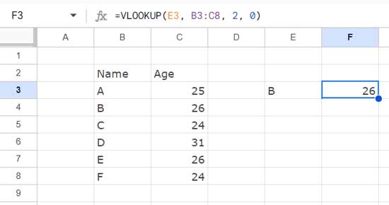
This formula follows the syntax:
VLOOKUP(search_key, range, index, [is_sorted])Where:
search_key:E3range:B3:C8index:2(result column in the range)is_sorted:0. It represents an exact match of thesearch_key(you can specify FALSE as well)
To retrieve two values, the ages of multiple persons in our context, specify their names in cells E3:E4 and use the following formula:
=ARRAYFORMULA(VLOOKUP(E3:E4, B3:C8, 2, 0))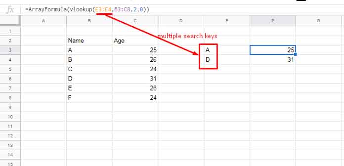
Note: If you hardcode the criteria instead of specifying them as E3:E4, use the VSTACK function as shown below:
VSTACK(search_key1, search_key2, ...)This example demonstrates how to retrieve multiple values using multiple search keys in VLOOKUP.
Using VLOOKUP to Retrieve All Values from the Matching Row (Using Multiple Column Indexes)
Sample Data:
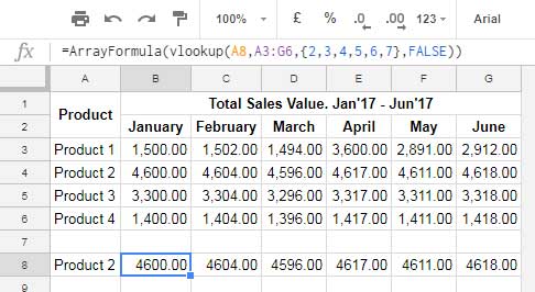
In the following example, I have product names in column A and sales from the first half of the year 2017 in columns B to G.
The actual range for lookup is A3:G6. Please refer to the screenshot provided below.
Lookup:
Enter the product name to search in cell A8.
To search it and return sales values from Jan to Jun, you can use the following VLOOKUP formula in cell B8.
=ARRAYFORMULA(VLOOKUP(A8, A3:G6, {2, 3, 4, 5, 6, 7}, 0))This example demonstrates how to retrieve multiple values using multiple index numbers in VLOOKUP.
Formula Explanation
In this example, the search key is from cell A8, which is used to search for the product name in the first column within the range A3:G6.
The match is found in cell A4, so the values from cells B4 to G4 in the same row are returned.
This demonstrates the use of the VLOOKUP formula to return all or selected values from a row based on a match in the first column of that row.
How Do These Multiple Values (Multiple-Column Indices) in VLOOKUP Work?
When you want to return a single value using VLOOKUP, you can use a formula similar to the one below:
=VLOOKUP(A4, A3:G6, 2, FALSE)The above VLOOKUP formula will find the search key in cell A4 and return the value from the second column in the same row.
When you want to return multiple values using VLOOKUP, you should use multiple column indexes within curly braces, as shown below:
{2, 3, 4}This creates an array that can return multiple column values in Google Sheets, specifically values from columns 2, 3, and 4. However, do not use the formula as follows:
=VLOOKUP(A4, A3:G6, {2, 3, 4}, FALSE)We have utilized curly braces to generate an array within the VLOOKUP formula. However, VLOOKUP is not an array formula by default.
Therefore, we should additionally use an ARRAYFORMULA function with the above formula. The final formula will be as follows:
=ARRAYFORMULA(VLOOKUP(A4, A3:G6, {2, 3, 4}, FALSE))This way, you can return multiple values using VLOOKUP in Google Sheets.
VLOOKUP Array Formula with Multiple Search Keys and Column Indexes
We have seen the use of VLOOKUP with ARRAYFORMULA in Google Sheets.
In the first set of examples, we used more than one search key from the same column to return an array output. In the second example, we specified multiple column indexes to return an array output.
Can we combine them both to get a 2D array result? The answer is yes.
In the last example, if you want to look up ‘Product 2’ and ‘Product 4’ entered in cells A8 and A9, you can use the formula below. It will return the values from the monthly columns.
=ARRAYFORMULA(VLOOKUP(A8:A9, A3:G6, {2, 3, 4, 5, 6, 7}, 0))As a side note, this type of 2D array result is not supported in XLOOKUP, another new lookup function, in the regular way.
But keep in mind that XLOOKUP is a newer and potentially better alternative for some VLOOKUP use cases. This is because XLOOKUP offers more flexibility due to its ability to use separate lookup and result ranges.
Unlike VLOOKUP, which is restricted to searching only the first column of a range (though this can be overcome with workarounds), XLOOKUP allows you to search in any column.
This can significantly simplify formulas, especially when working with complex data structures.


Great discussion. How would this work on using the Importrange function?
How would it be written in my case, where I have up to 30 columns to search?
Hi, JB9,
That might be possible. I require a sample Sheet to offer any possible solution.
Hello, I have read lots of your guides, but I am lost.
I have two sheets.
I want to bring all the rows that contain the matching word from Sheet 2 to Sheet1.
So if I have in Sheet 2:
Column 1 | Column2
Shakira | Blue
Shakira | Orange
Britney | Pink
Britney | Red
Shakira | Yellow
I want to have it in Sheet 1.
Column 1 | Column 2
Shakira | Blue, Orange, Yellow.
Britney | Pink, Red
Hi, Felipe Andres,
You can use this formula in Sheet1.
=textjoin(", ",true,filter(Sheet2!B:B,Sheet2!A:A=A2))Then drag it (copy-paste) down.
Hi Prashanth,
Thanks so much for the quick reply! This is EXACTLY what I was looking for – I really appreciate your help!!!
Also – I realized I left a duplicate comment on your thread. Sorry about that, and feel free to ignore it.
Isabel
Hello,
Is it possible for the ‘Filter’ function to ignore parameters when they are blank?
I’m trying to create a tool that returns a list of names that matches two criteria: State of residence, and Enrollment in a program (see example link below)
Thanks so much in advance!
Hi, Isabel,
Yes! We can do that in multiple ways in Google Sheets. I have copied your sheet as its sharing setting doesn’t allow me to put my formula.
I’ll leave the example ASAP below. Please stay tuned!
Update:
Please find my related tutorial here – IF Statement within Filter Function in Google Sheets.
Based on that, you can use the following formula.
=filter('Source Data'!A2:A,if(B2="",T('Source Data'!B2:B)<>"",'Source Data'!B2:B=B2),if(B3="",T('Source Data'!C2:C)<>"",'Source Data'!C2:C=B3))Other Formula Suggestions:
Option 1:
=filter('Source Data'!A2:A,regexmatch('Source Data'!B2:B&'Source Data'!C2:C,textjoin("",true,B2:B3)))Option 2:
=filter('Source Data'!A2:A18,if(B2="",'Source Data'!B2:B18<>"",'Source Data'!B2:B18=B2),if(B3="",'Source Data'!C2:C18<>"",'Source Data'!C2:C18=B3))Hello,
I’m trying to modify your formula to return data for multiple lines.
There are duplicate entries for the primary cell being used in the Vlookup. Would it be possible to use a similar formula to do this?
For example – if “Richard” showed up multiple times on the primary column, and I wanted to see all entries in the column range that the Vlookup is searching?
Hi, James,
You can try the Filter function.
For further assistance, please make a demo sheet and share it below. I won’t publish the address of the Sheet.
Hi there. Thanks for this very helpful article. I have a question, however: how to proceed if I wish to return multiple columns over many rows of data?
Example:
ArrayFormula(vlookup(E3:E4,B3:C8,{2,3,4},0))I wish to use a similar lookup in my scenario but cannot seem to get this to work.
Hi, Daniel Orr,
The above formula won’t work as there are only two columns in the ‘range’ and that should be specified as
{1,2}, not as{2,3,4}.So this Vlookup formula may work.
=ARRAYFORMULA(vlookup(E3:E4,B3:C8,{1,2},0))