Why should one use the IF logical statement within the Filter function in Google Sheets? Let me start this tutorial by answering this question I mean the IF and Filter combination use in Google Sheets.
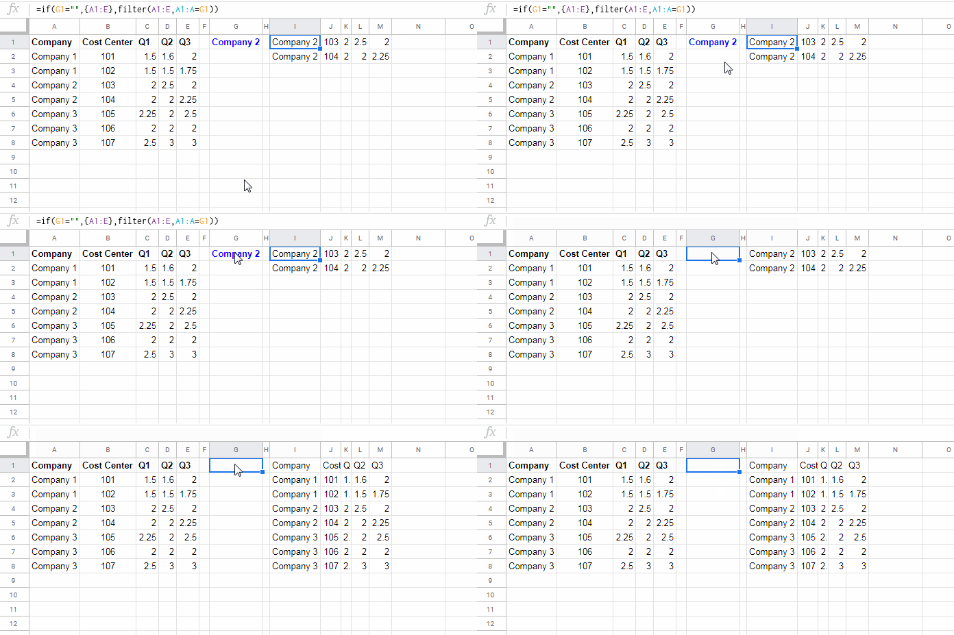
The sole purpose of this type of filtering is to skip filtering a table if the condition aka criterion is blank.
Normally if the criterion is blank, then the Filter formula would filter rows containing blank cells in the corresponding column.
Assume I have a table with 5 columns in the range Sheet1!A1:E and I want to filter this table using a criterion in Sheet1!G1.
Column A in the said table contains company names. In cell G1 there is one company name. So we will normally use this FILTER (in cell I1).
=filter(A1:E,A1:A=G1)Delete the criterion/condition in cell G1. The formula would return blank or rows from the table that contain blank values (null) in column A.
If the criterion is empty, then what I want is the entire table as the filtered output. This also we can sort out using an IF statement outside the above Filter formula.
=if(G1="",{A1:E},filter(A1:E,A1:A=G1))Note: The {A1:E} can be replaced by ArrayFormula(A1:E). Both, the Curly Braces and the ArrayFormula function returns an array.

But what about two conditions in Filter?
Then it’s better to use the IF statement within the Filter function in Google Sheets, not outside as above.
In this tutorial you can learn this IF and Filter combination use in Google Sheets.
How to Use IF Function within the Filter Function in Google Sheets
The use of this type of combination is useful when there is more than one condition. Even if you have a single condition as above, we can apply this logic.
Yes! Let’s first replace our earlier formula in this new way (approach).
Single Condition IF and Filter Combination in Google Sheets
Here first I am going to give you the IF and Filter combination use as an alternative to the just above formula.
=filter(A1:E,if(G1="",n(A1:A)<>"",A1:A=G1))I know most of you can read/understand the above formula with ease. A few of you may wonder about the role of N function in the formula. If so read the explanation below.
Formula Explanation
The IF statement used within the Filter formula tests whether the criteria cell G1 is blank or not. It works like this.
Syntax:IF(logical_expression, value_if_true, value_if_false)logical_expression – G1=""
value_if_true – n(A1:A)<>""
value_if_false – A1:A=G1
It says every thing.
If cell G1 is empty (value_if_true), then the IF feeds n(A1:A)<>"" to the Filter formula like;
=filter(A1:E,n(A1:A)<>"")That means ‘all the rows in the range’ because n(A1:A) returns a range with 0’s. We can replace n(A1:A) in the Filter formula with ROW(A1:A) too.
If cell G1 is not empty (value_if_true), then the IF feeds A1:A=G1 to the Filter formula like;
=filter(A1:E,A1:A=G1)Multiple Condition IF and Filter Combination in Google Sheets
In this case, let’s forget about using the IF statement outside the Filter function in Google Sheets. Here the use of IF statement within the Filter is more practical.
This also answers your following queries.
- How to skip filtering a column if the corresponding criterion is blank in Google Sheets?
- How to skip/ignore filtering a column if the drop-down criterion is blank in Google Sheets?
Actually answers to the above both questions are the same. Just read on to understand it.
Example
This time we have two conditions. One is in cell G1 that is the ‘Company’ name and another one is in cell G2 that is the ‘Cost Center’.
Further this time instead of directly entering the criteria, we can use data validation drop-down in these two cells.
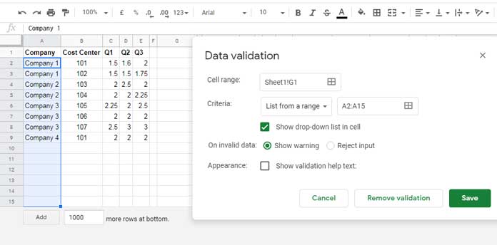
Click cell G1 and click Data > Data validation. Please follow the settings on the screenshot below.
Note: The sample data in A2:E has also been slightly modified.

Then click cell G2 and click Data > Data validation. The settings are similar to the first drop-down in cell G1. Here you must replace A2:A15 with B2:B15 and click ‘Save’.
Let’s start writing the formula (in cell I2) that contains multiple IF statements within the Filter function in Google Sheets.
Here is that formula in cell I2.
=filter(A1:E,if(G1="",n(A1:A)<>"",A1:A=G1),if(G2="",n(B1:B)<>"",B1:B=G2))Actually the above combination formula is an advanced form of the following formula.
=filter(A1:E,A1:A=G1,B1:B=G2)How Does this Formula Work?
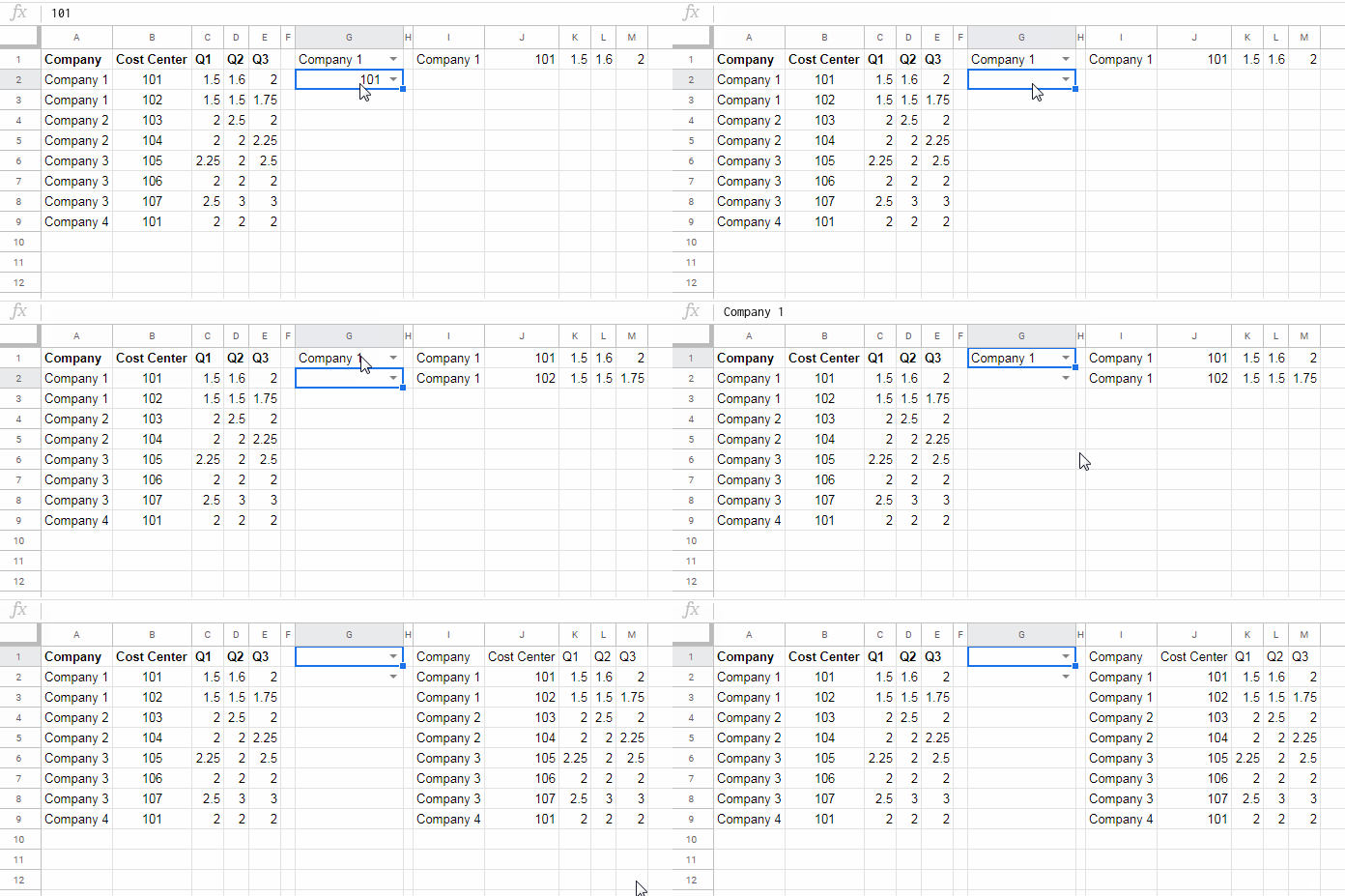
- G1 = “Company 1” and G2 = 101 (two conditions to filter).
- The formula returns the rows wherever column A matches ‘Company 1″ and column B matches 101.
- Hit the ‘Delete’ button in cell G1 (G1 is blank, G2 is 101).
- The formula would return wherever column B matches 101.
- Hit the ‘Del’ button in cell G2 (both G1 and G2 are blank).
- The formula would return the entire table as it is.

Conclusion
If you want to use one more (third) condition, use one more IF statement.
If the conditions are from the same column as “Company 1” in cell G1 and “Company 2” in cell G2, then use your regular Filter (given below). The IF and Filter function combination are not required.
=filter(A1:E15,regexmatch(A1:A15,textjoin("|",1,G1:G2)))Are you new to this type of, I mean using Regexmatch, Filter formula? Please see the third topic under “Resources” below.
Resources:
- Google Sheets: How to Get an All Selection Option in a Drop-down.
- Filter Rows if Search Key Present in Any Cell in that Rows in Google Sheets.
- Regexmatch in Filter Criteria in Google Sheets [Examples].
- Filter Based on a List in Another Tab in Google Sheets.
- Two-way Filter in Google Sheets [Dynamic Vertical and Horizontal Filter].
- How to Repeat Group Labels for Filtering in Sheets.
- Filter Out Matching Keywords in Google Sheets – Partial or Full Match.
- Comma-Separated Values as Criteria in Filter Function in Google Sheets.
- Filter Values Between Two Group Headers (Titles) in Google Sheets.


