You can use the REGEXMATCH function in the FILTER function criteria in Google Sheets to apply more specific filter conditions.
It helps you apply case-sensitive filtering and partial matches since the FILTER function doesn’t support case sensitivity or wildcard characters.
REGEXMATCH is a text function, so you should use it to filter based on text criteria. If you have a mixed data type column and want to include numbers as well, format the column to text by applying Format > Number > Plain Text.
Let’s learn how to use the FILTER function in combination with the REGEXMATCH function with the help of a few examples.
Using REGEXMATCH in FILTER Criteria for Partial Matches
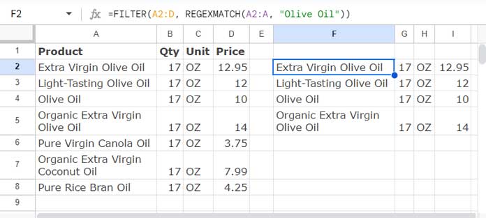
For this test, let’s use the following sample data in the range A1:D. For filtering, we will use only A2:D, excluding the header row.
| Product | Qty | Unit | Price |
| Extra Virgin Olive Oil | 17 | OZ | 12.95 |
| Light-Tasting Olive Oil | 17 | OZ | 12 |
| Olive Oil | 17 | OZ | 10 |
| Organic Extra Virgin Olive Oil | 17 | OZ | 14 |
| Pure Virgin Canola Oil | 17 | OZ | 3.75 |
| Organic Extra Virgin Coconut Oil | 17 | OZ | 7.99 |
| Pure Rice Bran Oil | 17 | OZ | 4.25 |
As you can see, our data comprises a list of different virgin oils and their prices. The first column contains the virgin oil names. Let’s see how to apply different conditions in this column.
The challenge here is to partially match text (substring match) in column A and filter the table.
The following examples explain how to properly use the REGEXMATCH function in the FILTER function criteria part.
Example 1: Partial Match of Single Criterion
The following formula filters the range A2:D wherever A2:A matches “Olive Oil”. It’s a partial, case-sensitive match.
=FILTER(A2:D, REGEXMATCH(A2:A, "Olive Oil"))This formula follows the syntax FILTER(range, condition1, [condition2, …]) where range is A2:D and condition1 is the REGEXMATCH formula.
The FILTER function filters the rows wherever the REGEXMATCH function returns TRUE.
Note:
The REGEXMATCH usually requires ARRAYFORMULA when testing values in a range. But within FILTER, it’s not applicable.
Example 2: Partial Match of Multiple Conditions
To filter rows wherever the range A2:A matches “Olive Oil” or “Coconut Oil”, use the following formula:
=FILTER(A2:D, REGEXMATCH(A2:A, "Olive Oil|Coconut Oil"))This is also case-sensitive. You can add more conditions by separating each condition with a pipe delimiter (|).
Controlling Case-Sensitivity
As mentioned earlier, both of the above formulas are case-sensitive. You can make them case-insensitive as follows:
=FILTER(A2:D, REGEXMATCH(A2:A, "(?i)Olive Oil"))
=FILTER(A2:D, REGEXMATCH(A2:A, "(?i)Olive Oil|Coconut Oil"))
Using REGEXMATCH in FILTER Criteria for Exact Matches
For example, if column A contains various fruit names and you want to filter only “apple”:
=FILTER(A:A, REGEXMATCH(A:A, "(?i)^apple$"))This is a case-insensitive formula that exactly matches “apple” in column A and filters those rows.
In the REGEXMATCH regular expression, ^ asserts the position at the start of a line and $ at the end of the line.
Here is one more example of using REGEXMATCH in FILTER criteria with the exact match of multiple criteria:
=FILTER(A:A, REGEXMATCH(A:A, "(?i)^apple$|^orange$|^mango$"))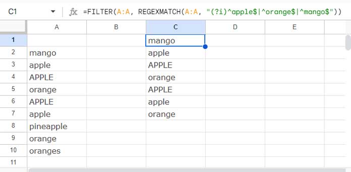
Resources
- REGEXMATCH in SUMIFS and Multiple Criteria Columns in Google Sheets
- REGEXMATCH Dates in Google Sheets – Single/Multiple Match
- How to Use REGEXMATCH in AVERAGEIF in Google Sheets
- Case-Insensitive REGEXMATCH in Google Sheets (Part or Whole)
- NOT in REGEXMATCH and Alternatives in Google Sheets
- Matches Regular Expression Match in Google Sheets QUERY


While the use of RegexMatch in the Filter is a very sleek way but I have observed that it fails if there is
( )i.e. bracket in the comparison text strings.The possibility of such oversight increase if the comparison text is a formula. I am sure there must be a few more unacceptable characters.
In such cases
=i.e. equality operator works well for comparison.Hi, S k Srivastava,
You should escape such special characters using the
\(backslash).Eg:
In cell D6 the string is “expert(sheets)”.
To match this string we can use the following RegexMatch formula.
=regexmatch(D6,"expert\(sheets\)")If you want to escape a backslash itself, then use the double backslash.
Eg.
String:
expert\sheets\Formula:
=regexmatch(D6,"expert\\sheets\\")The code is great, but be careful with the open- and closed-quotes if you’re copying and pasting. You’ll get a “formula parse error” if you copy the quotation marks directly. Instead, just delete the double-qoutes and enter them manually from your keyboard. Otherwise, good job!
Hi, Aaron Simmons,
Thanks for your valuable feedback!