Why should one use Regexmatch in Averageif function in Google Sheets?

The Regexmatch will help us to use multiple text conditions in one column in the Averageif function in Google Sheets. That’s my simple answer to the above question.

Yep! Averageif is capable of handling multiple text conditions in one column.

As per the Averageif syntax, which is as follows, we can use only one criterion in the criteria_range.

AVERAGEIF(
     criteria_range,
     criterion,
     [average_range]
)

But by using the Regexmatch function in the criteria_range argument, we can include multiple conditions in Averageif.

In addition to this, we can use the Regexmatch in Averageifs for the same purpose.

Any Alternatives?

Regarding alternatives, no doubt, there are so many!

We can use Query as an alternative to the above combination since Query has the AVG function as well as the MATCHES regular expression match in it.

Further, we can also use the combination of Average + Filter + Regexmatch or the database function DAVERAGE.

Let’s go to some examples to all the above starting with the Regexmatch in Averageif in Google Sheets.

Regexmatch in Averageif in Google Sheets

Enter the following data in A1:B9 in a Google Spreadsheet file.

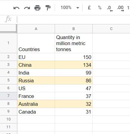
To find the average of the values (quantities in million metric tonnes) in B2:B9, no doubt, we can use the below Average formula.

=average(B2:B9)

I just want to find the average of the values in B2:B9, if the values in A2:A9 are “China”, “Russia”, or “Australia” (rows highlighted in light yellow).

Here comes the use of the Regexmatch in Averageif in Google Sheets.

Here is the formula.

=ArrayFormula(
     averageif(
        regexmatch(A2:A,"Australia|Russia|China"),
        TRUE,
        B2:B
     )
)

This formula would return 84 as the average which is the average of the values corresponding to the above country names.

How does this Regexmatch formula work within Averageif in Google Sheets?

Actually the Regexmatch matches the criteria “Australia”, “Russia”, and “China” in A2:A and returns TRUE in matching rows and FALSE in all the other rows.

Eg.:

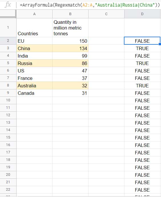
The above Regexmatch formula is the criteria_range in the Averageif.

Since the criteria_range contains Boolean TRUE or FALSE values, the criterion should be TRUE. The average_range is no doubt B2:B.

Regexmatch in Averageifs in Google Sheets

We can follow the same above logic to use the Regexmatch text function in Averageifs in Google Sheets.

To learn the use first see the Averageifs syntax in Google Sheets.

AVERAGEIFS(
     average_range,
     criteria_range1,
     criterion1,
     [criteria_range2, …],
     [criterion2, …]
)

Here the average_range comes first which is B2:B. The second argument, i.e. criteria_range1, is our earlier Regexmatch formula and the criterion1 here is TRUE.

Here is the Averageifs formula as per the above explanation.

=ArrayFormula(
     averageifs(
        B2:B,
        regexmatch(A2:A,"Australia|Russia|China"),
        TRUE
     )
)

Yes! You just need to alter the arguments used in Averageif here.

This way we can use Regexmatch in the Averageifs function in Google Sheets.

QUERY AVG function and Match Alternative

When you want to use Averageif or Averageifs with multiple conditions in one column you can depend on Query too.

See the formula first.

=query(
     A1:B,
     "Select avg(B) where A matches 'Australia|Russia|China' label avg(B)''",1
)

There are three Query clauses in the above formula and they are SELECT, WHERE, and LABEL (the last clause is optional though).

In these three, the SELECT clause selects the column (we can say the average_range column) to find the average.

In WHERE clause we use the MATCHES regular expression to match multiple criteria in column A (we can say criteria_range).

I am not going into much details as the above Query formula alternative to Averageif multiple criteria in one column is self-explanatory.

There are two more simple alternatives to the above Regexmatch in Averageif/Averageifs use in Google Sheets.

Additional Tips

Before winding up here are the said two simple solutions. First, I am going to use the combination of Average, Filter, and Regexmatch.

When you go through the sample data, you can understand one thing. Column A contains some country names and column B contains some production quantity in million metric tonnes.

Here, first we should filter the production quantities for the countries “Australia”, “Russia”, and “China”.

As explained earlier in one of my Google Sheets tutorial titled Regexmatch in Filter Criteria in Google Sheets, we can use the below formula for the said filtering.

=FILTER(
     B2:B,
     regexmatch(A2:A,"Australia|Russia|China")
)

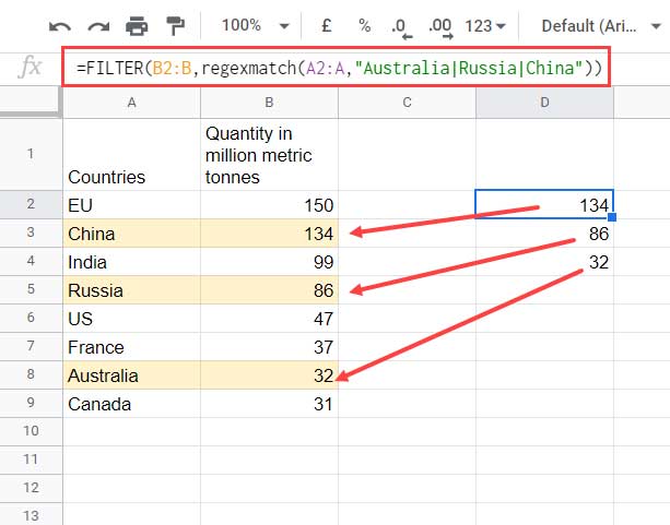
Then simply wrap the formula with the Average function.

=average(
     filter(
        B2:B,
        regexmatch(A2:A,"Australia|Russia|China")
     )
)

Here is the next alternative.

If you have a title row in your data similar to the row#1 (A1:B1) in my sample data range, then I suggest to you to use the DAVERAGE as below.

=daverage(
     A1:B,
     2,
     {"Countries";"Australia";"Russia";"China"}
)

It’s an elegant alternative solution to Averageif with multiple conditions in one column.

You May Like: The Ultimate Guide to Using Criteria in Database Functions in Google Sheets.

Hope you have learned how to use Regexmatch in Averageif in Google Sheets and also three useful alternatives.

That’s all. Enjoy!