The DAVERAGE function in Google Sheets is useful for calculating averages when your data is structured or when using Google Sheets tables.
Structured data refers to data organized like a database table, where columns are labeled (i.e., a range with a header row). In structured data, there should be no merged cells within the range. Google Sheets tables (Insert > Table) are also considered structured.
If your data is structured, you can use the DAVERAGE function instead of the AVERAGE, AVERAGEIF, or AVERAGEIFS functions.
Database functions, including DAVERAGE, can enhance data processing and analysis. Therefore, whenever possible, structure your data accordingly and use relevant database functions for aggregation and lookup tasks.
Syntax of the DAVERAGE Function in Google Sheets:
DAVERAGE(database, field, criteria)Arguments:
database: The range containing the data to be analyzed. It must be structured, meaning each column should have unique labels in the first row.field: The column number or label of the column containing the values to be averaged.criteria: The conditions to filter the database values before performing the calculation.
Examples
I will include tips on using different types of criteria in the example formulas below. Take your time to complete all the examples on your sheet.
The sample data in A1:D13 includes the date of supply in column A, material description in column B, unit in column C, and quantity in column D.
DAVERAGE with Single Criteria
Let’s start with a basic example of the DAVERAGE function in Google Sheets.
All database functions in Google Sheets, including DAVERAGE, take three arguments: database, field, and criteria. I have explained this above, and I’ve highlighted the first and last components in the screenshots below.
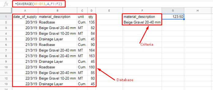
In this data, I want to find the average of the “qty” in column 4.
You can use either of the following formulas to find the average quantity for the product “Beige Gravel 20-40 mm”:
=DAVERAGE(A1:D13, 4, F1:F2)or
=DAVERAGE(A1:D13, "qty", F1:F2)What’s the difference between these two formulas?
In the second formula, you use the field label, while in the first formula, you use the column number.
Please note that the criteria range, F1:F2, is also structured.
The DAVERAGE formula above is equivalent to the following AVERAGEIF formula, for your reference:
=AVERAGEIF(B2:B13, F2, D2:D13)For quick reference, here is the syntax for AVERAGEIF in Google Sheets:
AVERAGEIF(criteria_range, criterion, [average_range])I highly recommend using database functions with structured data.
In DAVERAGE, as mentioned, you must use all three arguments: database, field, and criteria. You might wonder:
“I just want to find the average of the ‘qty’ column. I don’t want the formula to filter the data using any criteria. What’s the solution?”
The following example shows how to use the DAVERAGE function without criteria in Google Sheets.
DAVERAGE without Criteria
As mentioned, you must include all three arguments in the DAVERAGE formula. However, to skip filtering by criteria, simply leave the criteria cell blank.
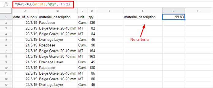
Here is the equivalent AVERAGE formula:
=AVERAGE(D2:D13)DAVERAGE with Multiple Criteria
I like how DAVERAGE manages multiple criteria. It’s simple to apply and easy to interpret when revisiting it later.
Here’s how you can include multiple criteria in the formula:
=DAVERAGE(A1:D13, 4, F1:F2)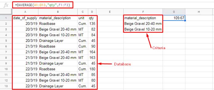
In this example, F1 contains the field label, while F2 and F3 contain the material descriptions as criteria.
The multiple criteria come from the same field, so you only need to enter each criterion one below the other.
If you’re looking for an alternative to the DAVERAGE formula, I suggest using the following formula:
=ArrayFormula(AVERAGEIFS(D2:D13, (B2:B13=F2)+(B2:B13=F3), ">0"))However, this approach is not straightforward since the conditions are from the same column.
Using Comparison Operators with the DAVERAGE Function in Google Sheets
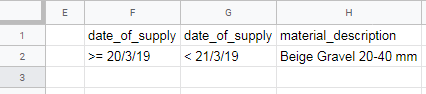
In the example below, I demonstrate how to use comparison operators in the DAVERAGE function. Additionally, note that there are multiple criteria from two different fields: date of supply and material description. We will apply the comparison operators to the date field.
=DAVERAGE(A1:D13, 4, F1:G2)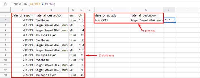
Since the criteria come from two different fields, you can also use AVERAGEIFS:
=AVERAGEIFS(D2:D13, A2:A13, F2, B2:B13, G2)I understand that another example may help clarify how to use comparison operators with the DAVERAGE formula in Google Sheets.
Please refer to the image below for further illustration. I won’t go into more details or formula explanation here.

Hardcoding Criteria in the DAVERAGE Function
I am not in favor of hardcoding criteria within database functions because it makes the formula complex. DAVERAGE is no exception. However, for the sake of completeness, here’s an example.
Using curly brackets, we can create virtual arrays in Google Sheets. If you’re familiar with this, it will make things much easier. Assume the following are the criteria you want to use in DAVERAGE (based on the previous example).
You can create this criteria range as a virtual array using curly braces, as shown below:
={
   "date_of_supply", "date_of_supply", "material_description";
   ">= 20/3/19", "< 21/3/19", "Beige Gravel 20-40 mm"
}
In the formula, commas separate the values into columns, while semicolons separate them into rows.
Alternatively, you can use a combination of the VSTACK and HSTACK functions:
=VSTACK(
   HSTACK("date_of_supply", "date_of_supply", "material_description"),
   HSTACK(">= 20/3/19", "< 21/3/19", "Beige Gravel 20-40 mm")
)
I will use this virtual criteria range in a formula.
In the first formula, the criteria are located in the range F1:H2:
=DAVERAGE(A1:D13, 4, F1:H2)Now, observe the same formula, but this time using the virtual array:
=DAVERAGE(A1:D13, 4, {"date_of_supply", "date_of_supply", "material_description"; ">= 20/3/19", "< 21/3/19", "Beige Gravel 20-40 mm"})I don’t prefer using criteria in this manner with the DAVERAGE function in Google Sheets.
Resources
- The Ultimate Guide to Using Criteria in Database Functions in Google Sheets
- Exact Match in Database Functions in Google Sheets – How-To
- How to Use the DSUM Function in Google Sheets
- How to Use the DPRODUCT Function in Google Sheets
- How to Use DCOUNT and DCOUNTA Functions in Google Sheets
- How to Use the DMAX Function in Google Sheets
- DMIN Function in Google Sheets – How to and Criteria Usage Tips
- Standard Deviation – DSTDEV Database Function in Google Sheets
- DGET Array Formula to Run Down a Column in Google Sheets
- How to Use the DSTDEVP Function in Google Sheets
- How to Use the DVAR Database Function in Google Sheets
- DVARP Function for Conditional Variance in Google Sheets


