This tutorial explains how to use the DVARP function to calculate the conditional variance of an entire population in Google Sheets.
Overview
The DVARP function calculates the variance, a measure of variability, based on a specified population. In Google Sheets, you can apply this function to a field containing multi-row records.
While it’s common to arrange your data in a database table format, it’s not strictly necessary in Google Sheets, as you can create virtual arrays to meet this requirement.
There are two database functions in Google Sheets for variance calculation: DVAR and DVARP. While DVAR is designed for use with a sample of the population, DVARP is intended for the entire population.
DVARP Function Syntax and Arguments
Syntax: DVARP(database, field, criteria)
Arguments:
1. Database
- This is the range of data to consider. The first row must contain labels for each column.
- For example, in the following table, the field labels are “Dog Breed,” “Height (mm),” and “Weight (lbs).”
| Dog Breed | Height (mm) | Weight (lbs) |
| Pug | 254 | 14 |
| Yorkshire Terrier | 203 | 7 |
| Papillon | 203 | 4 |
| French Bulldog | 305 | 16 |
| Labrador Retriever | 533 | 59 |
| Boxer | 536 | 66 |
| Pug | 280 | 17 |
| Pug | 260 | 15 |
| Pomeranian | 203 | 5 |
| Pomeranian | 178 | 3 |
| Pomeranian | 279 | 7 |
If your data lacks field labels, you can specify them virtually within the formula.
2. Field
- This indicates which column in the database to use for variance calculation. You can refer to it using either a text label or a numeric index (e.g., 2 for the “Height (mm)” column).
Example:
- Text Label Method:
=DVARP(database, "Height (mm)", criteria) - Numeric Index Method:
=DVARP(database, 2, criteria)
3. Criteria
- This specifies the conditions to filter the database before performing the calculation. At least one field label and one cell below it are required for the criteria range.
- If your data is unstructured and lacks a header row, you may need to use a workaround to specify criteria.
Examples of the DVARP Function
Example Data
Consider the database shown above, which includes a list of dog breeds in column A, their heights in column B, and weights in column C. The total number of records is 12, including the header row.
Using the DVARP Function
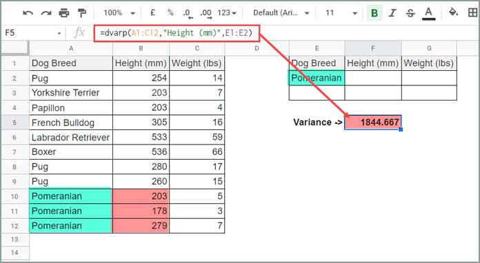
To extract records for “Pomeranian” and calculate the variance of their height in millimeters, you can use the following formula:
- Text Label Method:
=DVARP(A1:C12, "Height (mm)", E1:E2) - Numeric Index Method:
=DVARP(A1:C12, 2, E1:E2)
Multiple Criteria
To include both “Pomeranian” and “Yorkshire Terrier” in the criteria, add “Yorkshire Terrier” in cell E3 and modify the criteria range:
=DVARP(A1:C12, 2, E1:E3)Specifying Criteria Within the Formula
You can also specify criteria directly within the DVARP formula:
=DVARP(A1:C12, 2, {"Dog Breed"; "Pomeranian"; "Yorkshire Terrier"})For more information on using criteria, please refer to the Resources section at the bottom of this post.
Using DVARP Function with Missing Field Labels
If your data lacks field labels in the first row, the previous formulas may return a #VALUE! error. Here’s how to work around this:
=DVARP({" ", " ", " "; A2:C12}, 2, {" "; E2:E3})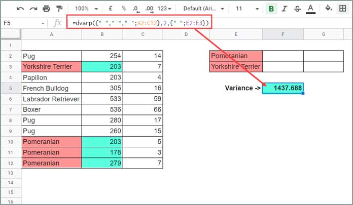
Criteria Hardcoded:
=DVARP({" ", " ", " "; A2:C12}, 2, {" "; "Pomeranian"; "Yorkshire Terrier"})Here, we add virtual space characters as field labels.
Additional Notes
- Using DVARP Without Criteria:
If you want to include all records in your calculation, specify one of the column references from the database. For example, to include all dog breeds, use:=DVARP(A1:C12, 2, A1:A12) - Handling Blank Cells:
The DVARP function will ignore records in the evaluation column that contain blank cells, text strings, TRUE, or FALSE. However, it will include zero values in the calculation.
Resources
You may find the following tutorial useful for further understanding:


