There are 12 database functions in Google Sheets that start with the letter ‘D.’ I have covered all of them in my Google Sheets functions guide. In this guide, I will focus primarily on correctly using criteria in database functions in Google Sheets.
All database functions, whether DSUM, DPRODUCT, or any other D function, share the same set of common arguments: database, field, and criteria.
Although this guide focuses on the criteria argument, it’s important to understand the other two arguments as well.
Database
The database is the range or array used for computation, and it must contain field labels in the first row (see the image below).
For example, if your range/array contains 4 columns, it means you have a database with four fields.
Field
The field argument indicates, except in DGET, which column contains the values to be aggregated. In DGET, the field represents the column from which the output will be returned.
To specify the field, you can use either the field label or the column number. In all the formulas used in this guide, I will be using the column number instead of the field label.
Criteria
Unlike other native spreadsheet functions, criteria in Database functions must be structured in Google Sheets. This means you need to include the field labels along with the criteria.
Our sample data includes “Customer Name,” “Inv. No.,” “Date,” and “Amount,” and is located in the range A1:D10.
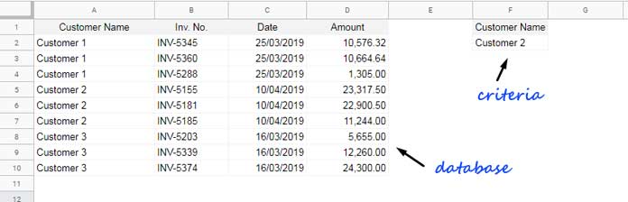
To apply a criterion in the “Customer Name” field, the criteria can be structured as an embedded array like F1:F2, where F1 contains “Customer Name” (the field label) and F2 contains “Customer 2” (the customer’s name).
Additionally, the criteria/conditions can be generated as an array using an array expression, such as:
={"Customer Name"; "Customer 2"}In this tutorial, I will explain in detail how to use criteria in database functions. I will cover how to properly embed criteria as well as how to generate complex criteria using array expressions.
Database Functions in Google Sheets with Single Criteria
First, let me share the common syntax for database functions. Replace function_name with the database function of your choice:
function_name(database, field, criteria)Single String Criteria
Database: For the sample database, refer to the range A1:D10 in the screenshot above.
Field: I am using the fourth column, i.e., the number 4 as the field.
Criteria: In the screenshot, I have embedded the criteria in the range F1:F2.
For this example, I am using the DSUM function:
=DSUM(A1:D10, 4, F1:F2)Here’s the same DSUM formula with criteria generated by an array expression:
=DSUM(A1:D10, 4, {"Customer Name"; "Customer 2"})This formula returns the sum of values in the “Amount” column (column 4), filtered based on the specified criteria.
Single Date Criteria
To test the usage of embedded criteria, enter “Date” in F1 and a specific date, such as 25/03/2019, in cell F2. The formula remains unchanged:
=DSUM(A1:D10, 4, F1:F2)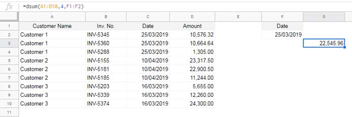
This formula will return the sum of amounts in rows that match the date in the “Date” column.
To use a date criterion as an array expression, it is preferable to use the DATE function with the syntax DATE(year, month, day), rather than hardcoding the date criterion directly:
=DSUM(A1:D10, 4, {"Date"; DATE(2019, 3, 25)})Single Numeric Criteria
To sum the values in field #4 where the invoice value is 6000.00:
Enter “Amount” in F1 and 6000 in F2, then use the following formula:
=DSUM(A1:D10, 4, F1:F2)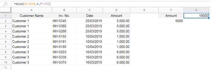
Here is the equivalent formula using an array expression:
=DSUM(A1:D10, 4, {"Amount"; 6000})With this, we conclude the basic usage of criteria in database functions in Google Sheets. Now, let’s move on to the more complex topic of multiple criteria.
Database Functions with Multiple Criteria in Google Sheets
In the earlier examples, I used the DSUM function. Regardless of which D function you use, the tips for applying criteria remain the same. For a change, let’s use DMAX here.
Multiple Conditions in the Same Field (Similar to OR Condition)
The following formula uses customer names in F2 and F3, with F1 containing the field label:
=DMAX(A1:D10, 4, F1:F3)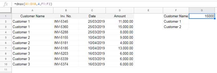
This formula returns the maximum value in column 4, filtering by customer names in column 1.
This is similar to using OR criteria since the conditions are from the same column—essentially stating “this or that.”
Alternatively, you can include the criteria directly in the formula:
=DMAX(A1:D10, 4, {"Customer Name"; "Customer 1"; "Customer 2"})Note that the semicolon separates the values into different rows in the same column. If you want to place conditions in two different columns, use a comma as the separator.
Note: The use of semicolons or commas might be affected by your locale settings. For more details, check out How to Use Curly Brackets to Create Arrays in Google Sheets.
Multiple Conditions from Different Fields (Similar to AND Condition)
Before moving on to the next example of using criteria in database functions in Google Sheets, it’s important to understand how to use array expressions to form multiple criteria.
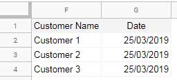
Suppose the image above shows our next embedded criteria range F1:G4. To use an array expression within the formula, follow these steps:
Step 1:
Create an array expression to place the values from F1:F4 into rows in the same column:
={"Customer Name"; "Customer 1"; "Customer 2"; "Customer 3"}Step 2:
Create an array expression to place the values from G1:G4 into rows in the same column:
={"Date"; DATE(2019, 3, 25); DATE(2019, 3, 25); DATE(2019, 3, 25)}Step 3:
Combine both arrays (from Step 1 and Step 2). Use a comma as the separator to create two columns:
={{"Customer Name"; "Customer 1"; "Customer 2"; "Customer 3"}, {"Date"; DATE(2019, 3, 25); DATE(2019, 3, 25); DATE(2019, 3, 25)}}You can use this array expression in the following formula:
=DSUM(A1:D10, 4, F1:G4)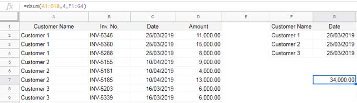
This formula filters the records for “Customer 1,” “Customer 2,” and “Customer 3” where the corresponding date in the “Date” column is 25/03/2019.
Equivalent Formula:
=DSUM(A1:D10, 4, {{"Customer Name"; "Customer 1"; "Customer 2"; "Customer 3"}, {"Date"; DATE(2019, 3, 25); DATE(2019, 3, 25); DATE(2019, 3, 25)}})Using Comparison Operators with Database Function Criteria
There are six comparison operators you can use with D Functions in Google Sheets:
=Equal to<Less than>Greater than<>Not equal to<=Less than or equal to>=Greater than or equal to
You don’t need to use the = operator with date or numeric criteria. However, use it with text criteria if you want an exact match, rather than a partial match.
For example, the criterion "Customer 1" will match both "Customer 1" and "Customer 11". To ensure an exact match, use the criterion "=Customer 1".
=DSUM(A1:D10, 4, {"Customer Name"; "=Customer 1"})When embedding criteria, you may not be able to start with = because it could be interpreted as a formula. To avoid this issue, start with an apostrophe (') followed by the equal sign and the criterion:
'=Customer 1Related: Exact Match in Database Functions in Google Sheets – How-To
You can use all the other comparison operators in numeric and date fields with database functions in Google Sheets.
I will provide examples using a date field.
Examples
Problem: Filter “Customer 2” in field 1 if the invoice dates are greater than 25/03/2019 in field 3, and then find the average in field 4.
To find the average in a database, you can use the DAVERAGE function. Enter “Customer Name” in F1 and “Date” in G1. Then enter “Customer 2” in F2 and “>25/03/2019” in G2.
Formula:
=DAVERAGE(A1:D10, 4, F1:G2)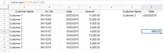
Equivalent Formula:
=DAVERAGE(A1:D10, 4, {{"Customer Name"; "Customer 2"}, {"Date"; ">" & DATE(2019, 3, 25)}})Similarly, you can use other comparison operators. For filtering a date range in database functions, follow this approach:
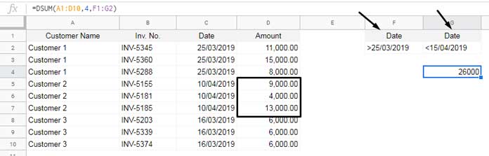
To filter records between the date range 25/03/2019 and 15/04/2019 (exclusive), and find the average of values in field 4:
Enter “Date” in F1 and G1. Then enter “>25/03/2019” in F2 and “<15/04/2019” in G2.
Using VSTACK and HSTACK in Database Function Criteria
In the examples above, we used curly braces for criteria with array expressions. Alternatively, you can use the VSTACK and HSTACK functions.
- VSTACK vertically combines values (for OR criteria).
- HSTACK horizontally combines values (for AND criteria).
OR Criteria:
=VSTACK("Customer Name", "Customer 1", "Customer 2")AND and OR Criteria:
=VSTACK(
   HSTACK("Date", "Date"),
   HSTACK(">" & DATE(2019, 3, 25), "<" & DATE(2019, 4, 15))
)
Resources
Here are some guides on using D functions in Google Sheets:


This was a great tutorial, thanks! However, I am having a problem. I have a table like this:
NAME|RANK|SALARY|MAX_SALARY
John Smith|Private|$40,000|DMAX FORMULA
Mary Jones|Captain|$90,000|DMAX FORMULA
Karl Wilson|Private|$38,000|DMAX FORMULA
What I want is for the value of the MAX_SALARY cell to equal the maximum salary for the RANK of each person.
So for John Smith’s DMAX FORMULA I tried
=DMAX(A1:C3,3,={"RANK";B2})figuring that this would look for the value of RANK = “Private” in all three rows, find two of them, and return the maximum (in this case $40,000).However, I’m getting a Formula Parse Error. Any idea what I’m doing wrong (or perhaps a better way to do what I want)?
Hi, David Rossien,
You were so close. Try this formula instead.
=dmax($A$1:$C$4,3,{"Rank";B2})Hi, David Rossien,
Additionally, we can make it a row-wise array formula using the new Named Function.
I’ll include it in my upcoming tutorial and let you know by updating this comment.
Update:- You can find the formula in this tutorial – How to Use the MAKEARRAY Function in Google Sheets.