The DMAX function in Google Sheets is a database function, while its alternative, MAXIFS, is statistical. So, which one should you choose?
DMAX and MAXIFS are popular spreadsheet functions for finding the maximum value based on specific conditions.
Additionally, you can use the QUERY function for the same purpose in Google Sheets, although it’s typically used for more advanced data manipulation.
DMAX or MAXIFS: which should you use for conditional max in Google Sheets?
If you’re unsure, here’s the answer.
First, ensure that you’re working with structured data. If so, DMAX is the clear choice.
In the following example, I have dates, delivery order numbers, material descriptions, and weight in metric tons (MT) in the range A1:D12. The first row contains the labels: Date, DO No., Material, and Wt in MT, respectively.
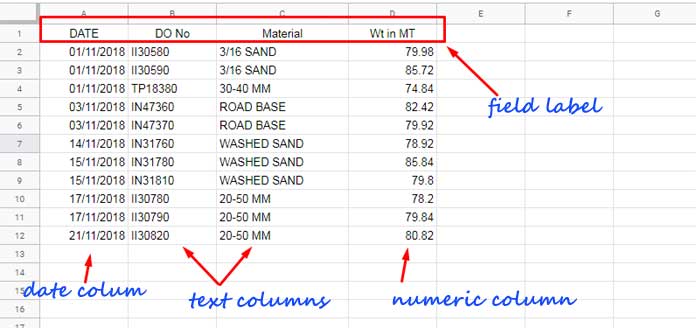
In this structured sample data, you can use DMAX to find the maximum value in column D.
Why is this considered structured data?
- There are no merged cells.
- The dataset has a top row with field labels.
If your data meets these criteria, then database functions like DMAX are appropriate. Also, note that tables (Insert > Table) are structured.
Before diving into how to use the DMAX function with examples, let me first explain the purpose of DMAX and its syntax.
Syntax, Arguments, and Purpose
The purpose of the DMAX function in Google Sheets is to return the maximum value from a database-like array (structured data) using a query-like filter.
Syntax:
DMAX(database, field, criteria)Arguments:
database– The table or range that contains the data to consider.field– Specifies the column in thedatabasefrom which the maximum value will be extracted. This can be the column label or the column number. I prefer using the column number.criteria– A structured range or array that defines the conditions to filter thedatabasebefore calculating the maximum value.
Examples of Using the DMAX Function in Google Sheets
Below, find a couple of examples of how to use the DMAX database function in Google Sheets.
DMAX Without Criteria in Google Sheets
If you exclude the criteria, the DMAX formula will return a #N/A error. This is because the function requires all arguments to be provided—none of them are optional.
So, how can you exclude criteria in a DMAX formula in Google Sheets?
You can use a formula like this:
=DMAX(A1:D12, 4, {"Material"; ""})Here, we include one of the field labels and leave the criterion blank, as shown in the example.
You can also use a cell reference for the criterion, but this can become confusing if the criteria field is a date column. Why?
Blank Date as Criteria in the DMAX Formula:
I have a two-column structured dataset, which is the output of the following GOOGLEFINANCE formula:
The formula in cell A1:
=GOOGLEFINANCE("NSE:HINDPETRO", "price", EDATE(today(),-12), today(), "DAILY")This formula returns the stock price of the ticker symbol “HINDPETRO” (NSE India) from the Google Finance database for the past 12 months. The first column contains dates, and the second column contains the closing prices, with labels “Date” and “Close.”
Enter the field label “Date” in cell E1 and leave the cell below empty. Use the following formula to get the maximum closing price:
=DMAX(A1:B, 2, E1:E2)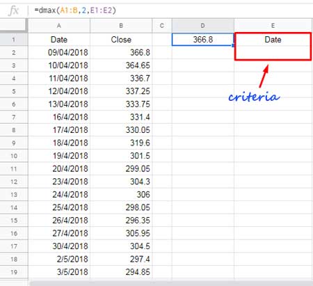
How do you hardcode the criteria range E1:E2 in the formula?
This approach won’t work: =DMAX(A1:B, 2, {"Date"; ""})
It’s a bit tricky! To exclude conditions, you can specify them as two virtual blank cells:
=DMAX(A1:B, 2, {IF(,,); IF(,,)})This method is applicable not only to date columns but also to numeric and text columns.
You can find more details here: Two Ways to Specify Blank Cells in Google Sheets Formulas.
Single Criterion (Cell Reference and Hardcoding)
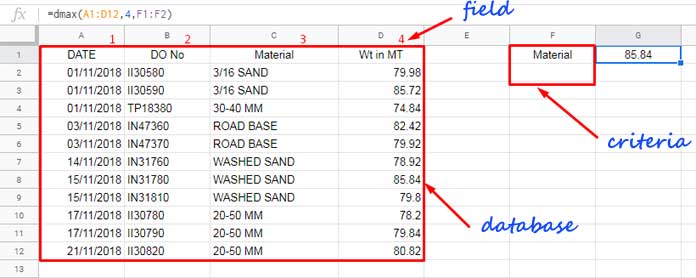
Let’s return to our sample data in A1:D12.
I want to find the maximum value for the material “3/16 SAND” to determine the highest quantity of this item shipped on any day.
To do this with hardcoding:
=DMAX(A1:D12, 4, {"Material"; "3/16 SAND"})If you prefer to use a cell reference for the criterion, enter “Material” in cell F1 and “3/16 SAND” in cell F2. Then, use the following formula:
=DMAX(A1:D12, 4, F1:F2)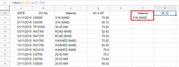
Multiple Criteria in the Same Field in the DMAX Function in Sheets
In the previous example, we found the maximum quantity of the item “3/16 SAND.”
Now, I want to find the maximum quantity for both “3/16 SAND” and “WASHED SAND.”
To do this, enter the new criteria in cell F2, and update the criteria range in the earlier formula to F1:F2:
=DMAX(A1:D12, 4, F1:F2)If you prefer to hardcode the criteria directly into the DMAX function, it gets a bit more complex:
=DMAX(A1:D12, 4, {"Material"; "3/16 SAND"; "WASHED SAND"})For a detailed explanation of this formula, you can refer to: The Ultimate Guide to Using Criteria in Database Functions in Google Sheets.
Multiple Criteria from Two Different Fields in the DMAX Function in Sheets
When conditions are based on two different fields, you can use the DMAX function as follows:
For example, enter the field labels “Date” and “Material” in cells F1 and G1, and place the corresponding criteria below these labels.
The DMAX formula below returns the maximum value for the material “3/16 SAND” shipped on 01/11/2018:
=DMAX(A1:D12, 4, F1:G2)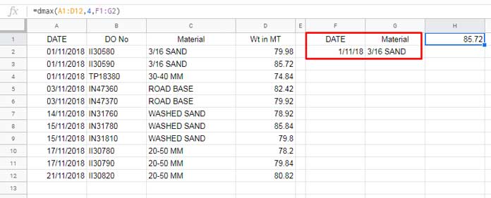
It’s straightforward, but understanding how to hardcode multiple criteria in the DMAX formula is essential.
Here’s how:
=DMAX(A1:D12, 4, {"DATE", "Material"; DATE(2018,11,1), "3/16 SAND"})Referencing or hardcoding criteria in Google Sheets database functions follow similar patterns.
If you have any doubts about this, you can refer to this tutorial: How to Properly Use Criteria in DSUM in Google Sheets [Chart] or the earlier mentioned resources.
I hope you found these DMAX function tips and tricks helpful. See you next time!


