You can track your financial portfolio in Google Sheets using the GOOGLEFINANCE function.
The GOOGLEFINANCE function allows you to retrieve live and historical stock prices, as well as currency exchange rates, directly from the Google Finance website. With this information, you can create a personalized financial portfolio tracker in Google Sheets.
However, do not rely solely on this function for tracking your investments. Numerous websites offer tools to monitor stock movements more comprehensively. Use this function for informational purposes only and not for making trading, financial, or investment decisions.
Before using the function, review the following points.
Things to Know Before You Start Using the GOOGLEFINANCE Function
You may encounter the function being unresponsive or returning #N/A errors due to various reasons:
- Incorrect Ticker: Ensure that the ticker symbol is correct. If a previously working ticker stops functioning, it may be due to internal errors beyond your control or changes in the listed company’s ticker.
- Market Information: The GOOGLEFINANCE function retrieves stock data directly from the Google Finance website.
- Data Delay for Current Prices: When fetching real-time data, there may be a delay of up to 20 minutes, as indicated by a notification bar at the bottom of the sheet.
- Exchange Codes and Delays: You can find more details about exchange codes and delay times in the Google Finance Data Listing and Disclaimers.
GOOGLEFINANCE Function: Syntax, Arguments, and Examples
Syntax:
GOOGLEFINANCE(ticker, [attribute], [start_date], [end_date|num_days], [interval])Ticker
In this syntax, the argument “ticker” represents the ticker symbol of the security to consider to get live or historical data.
You should use both the exchange symbol and ticker symbol for accurate results and to avoid the GOOGLEFINANCE function to judgement and to choose one for you.
Example:
=GOOGLEFINANCE("NSE:RELIANCE")This returns the real-time price quote for RELIANCE from the National Stock Exchange of India (NSE), as “price” is the default attribute.
Currency Exchange Rates:
To get currency exchange rates, use the “CURRENCY” prefix followed by the currency codes.
Example:
=GOOGLEFINANCE("CURRENCY:USDINR")This formula returns the exchange rate for 1 USD to INR.
For a list of currency codes, visit the ISO 4217 Wikipedia page.
Attribute for Real-Time Stock Data
For real-time stock data, you can specify one of the following attributes in the GOOGLEFINANCE function:
| Attribute | Description |
| price | The latest stock price, with a delay of up to 20 minutes. |
| priceopen | The stock price at market open. |
| high | The highest price reached during the current trading day. |
| low | The lowest price recorded during the current trading day. |
| volume | The total number of shares traded on the current day. |
| marketcap | The company’s market capitalization. |
| tradetime | The timestamp of the most recent trade. |
| datadelay | The delay duration of the real-time data feed. |
| volumeavg | The average daily trading volume. |
| pe | The ratio of the stock’s price to its earnings per share. |
| eps | The earnings generated per share of the stock. |
| high52 | The highest price of the stock over the past 52 weeks. |
| low52 | The lowest price of the stock over the past 52 weeks. |
| change | The price change since the previous day’s close. |
| beta | The stock’s volatility relative to the market. |
| changepct | The percentage change in price from the previous trading day’s close. |
| closeyest | The stock’s closing price on the previous trading day. |
| shares | The total number of shares currently outstanding. |
| currency | The stock’s pricing currency. (Note: Currency does not support attributes like high or low as it lacks trading sessions.) |
Example:
=GOOGLEFINANCE("NSE:RELIANCE", "high")This formula returns the highest price RELIANCE reached during the current trading day.
You can also input the ticker symbol and attribute in separate cells and reference them in the formula. For instance, if cell A1 contains NSE:RELIANCE and cell B1 contains high, you can write:
=GOOGLEFINANCE(A1, B1)Note: The function is case-insensitive.
Historical Stock Data: Attributes, Start Date, End Date, and Interval Parameters
For historical data, you can specify additional arguments like start_date, end_date, and interval.
| Attribute | Description |
| open | The stock’s opening price for the given date(s). |
| close | The stock’s closing price for the specified date(s). |
| high | The highest price recorded on the specified date(s). |
| low | The lowest price recorded on the specified date(s). |
| volume | The total number of shares traded for the specified date(s). |
| all | Includes all of the above data points. |
Ensure your formula has enough blank rows and columns to display all results, including headers and timestamps.
Example:
=GOOGLEFINANCE("NSE:RELIANCE", "open", DATE(2018,6,1), DATE(2018,6,10), "DAILY")This formula returns the opening prices of RELIANCE from June 1, 2018, to June 10, 2018.
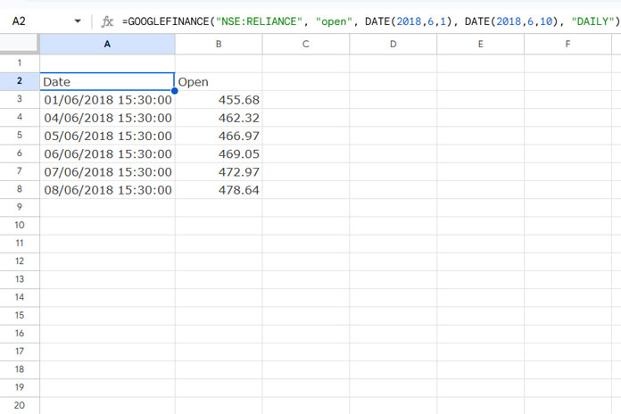
In this example, the interval is set to "DAILY". You can modify it to "WEEKLY" if you prefer weekly data instead.
Explanation of the Syntax:
- ticker:
"NSE:RELIANCE" - attribute:
"open" - start_date:
DATE(2018,6,1)(You can also write it as"2018-06-01"in ISO 8601 format.) - end_date:
DATE(2018,6,10)(Alternatively, use"2018-06-10"in ISO 8601 format.) - interval:
"DAILY"(Use"WEEKLY"for weekly intervals.)
If you prefer, instead of specifying an end_date, you can define the number of days from the start_date to retrieve data.
Attributes for Mutual Fund Data in GOOGLEFINANCE Function
| Attribute | Description |
| name | The name of the mutual fund. |
| closeyest | The closing price from the previous trading day. |
| date | The date when the net asset value (NAV) was reported. |
| returnytd | The return on investment since the beginning of the year. |
| netassets | The total value of the fund’s net assets. |
| change | The difference between the most recent reported NAV and the one immediately preceding it. |
| changepct | The percentage difference between the most recent and previous NAVs. |
| yieldpct | The distribution yield, calculated as the sum of the last 12 months’ income distributions (dividends and interest) and NAV gains, divided by the NAV at the end of the previous month. |
| returnday | The total return over one day. |
| return1 | The total return over one week. |
Example Formula:
=GOOGLEFINANCE("MUTF_IN:EDEL_LARG_MID_1D0HAMC","date")Additional Tips
Using Multiple Tickers in Real-Time Stock Data with Lambda
The GOOGLEFINANCE function is an array formula, even though it returns a single output for real-time stock data. This means you cannot directly specify multiple ticker symbols to get their real-time stock data all at once.
For example, if you want the real-time “price” of the tickers listed in range A2:A, you can enter the following formula in cell B2 and drag it down:
=GOOGLEFINANCE(A2, "price")Alternatively, if you have multiple tickers in a column and want to use them all without dragging the formula down, you can use the MAP and LAMBDA functions:
=IFNA(MAP(A2:A, LAMBDA(ticker, GOOGLEFINANCE(ticker, "price"))))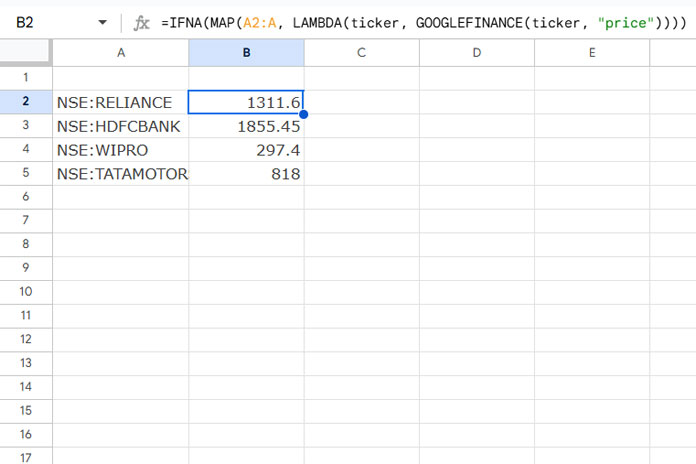
Removing Headers and Columns in Historical Data from GOOGLEFINANCE Output
Consider the following formula:
=GOOGLEFINANCE("NSE:RELIANCE", "close", "2024-12-01", 5)This formula returns the closing price of the stock starting from the specified date and for the next 5 days. To omit the header row from the output, you can use the following formula:
=LET(data, GOOGLEFINANCE("NSE:RELIANCE", "price", "2024-12-01", 5), CHOOSEROWS(data, SEQUENCE(ROWS(data)-1, 1, 2)))To select the price column, wrap the formula with CHOOSECOLS as follows:
=CHOOSECOLS(LET(data, GOOGLEFINANCE("NSE:RELIANCE", "price", "2024-12-01", 5), CHOOSEROWS(data, SEQUENCE(ROWS(data)-1, 1, 2))), 2)This formula will return only the price data without the header row.


Hi,
Can I use arrayformula with
=arrayformula(googlefinance(M2:M,"price"))It is only returning the 1st row.
Thanks
Hi, SPH,
It’s not possible as GoogleFinance itself is an array formula. If you use the start date and end date arguments, the formula would return an array result.
So in your case, you need to copy-paste the formula down.
Accurate information, Thanks team, you helped me a lot