When fetching historical data, if you use the start_date and end_date parameters, the GoogleFinance function would return two column data. This raises one question! That’s how to find the Max and Min values in GoogleFinance historical data?

If it’s a single column data, without any doubt, you can use the MIN or MAX functions. Even if it’s a two-column array, if any of the whole columns contain text values, the above functions will work.

But in Google Sheets, the GoogleFinance function returns two column data. In which the first column contains date time and the second column contains the historical values.

That’s why the question of how to find Max and Min values in GoogleFinance historical data become relevant.

To find Max and Min values in GoogleFinance, I have different formula options to present in front of you. You can prefer the easiest one from my formula suggestions.

Options to Find Max and Min Values in GoogleFinance Historical Data

You can use any of the below functions to apply Min and Max in multi-row historical data in Google Sheets.

1. Query.
2. DMAX/DMIN Database Functions.
3. MAX/MIN function with INDEX (combo formula).

First let me show you the structure of a Google Finance historical data output.

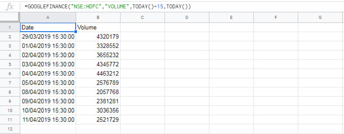
=GOOGLEFINANCE("NSE:HDFC","VOLUME",TODAY()-15,TODAY())

This GoogleFinance formula fetches the trading volumes for the last 15 days of the security “HDFC”. It’s historical data so it would return expanding output as below.

Two Column Historical Data:

In this, I have used the attribute “volume”. Other supported attributes in historical data are “open”, “close”, “high”, “low”, and “all”.

In this, other than the “all” attribute, all the attributes would return two column data as above.

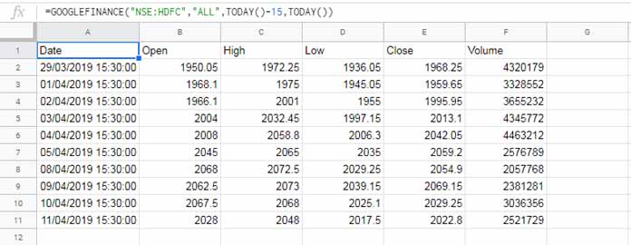
If you use the “all” attribute, it would return a multi-column output as below.

Multi-Column Historical Data:

Needless to say, the formula to retrieve Max and Min values in GoogleFinance historical data will vary in two columns as well as in multi-column outputs.

Finding Max Values in GoogleFinance Two Column Historical Data

Let me begin with the Query formula. I prefer the Query as it’s simple to read.

Query to Find Max Value in GoogleFinance Historical Data

Syntax:

QUERY(data, query, [headers])

Use the GoogleFinance historical data formula as your “data” in Query. We can use the Max aggregation function in “query”.

Formula:

=QUERY(GOOGLEFINANCE("NSE:HDFC","VOLUME",TODAY()-15,TODAY()),"Select Max(Col2) label Max(Col2)''",1)

You May Like: How to Sum, Avg, Count, Max, and Min in Google Sheets Query.

DMAX Database Function in GoogleFinance Historical Data (Multi-Row Data)

The GoogleFinance historical data is well structured as a database table. It has field labels in the first row. That makes the data eligible for using in DMAX function.

The field label for the first column is “Date”. But the field label for the second column depends on the attribute in use.

In my example, it’s “Volume” in the two column data. You can check the concerned screenshot above.

What I am trying to say is, in structured data, you can use the DMAX database function to return the Max value.

Syntax:

DMAX(database, field, criteria)

Formula:

=DMAX(GOOGLEFINANCE("NSE:HDFC","VOLUME",TODAY()-15,TODAY()),2,{"Date";">"&text("30/12/1899","dd/mm/yyyy")})

I have already explained this usage in my tutorial related to the DMAX function.

MAX and INDEX Combo to Find Max in Multi-Row Data

Formula:

=max(index(GOOGLEFINANCE("NSE:HDFC","VOLUME",TODAY()-15,TODAY()),0,2))

Here the INDEX formula (see that below) offsets 2 columns. So you will left with the second column.

=index(GOOGLEFINANCE("NSE:HDFC","VOLUME",TODAY()-15,TODAY()),0,2)

That means you can just wrap this Index formula with the regular Max function to find the max value.

Finding Min Values in GoogleFinance Two Column Historical Data

Here I am directly going to give you the three different formulas. These formulas have only one common difference with the above formulas. What’s that?

To find Min values from Google Finance historical Data, change the functions MAX with MIN as follows.

Query:

=QUERY(GOOGLEFINANCE("NSE:HDFC","VOLUME",TODAY()-15,TODAY()),"Select Min(Col2) label Min(Col2)''",1)

DMIN:

=DMIN(GOOGLEFINANCE("NSE:HDFC","VOLUME",TODAY()-15,TODAY()),2,{"Date";">"&text("30/12/1899","dd/mm/yyyy")})

MIN/Index:

=MIN(index(GOOGLEFINANCE("NSE:HDFC","VOLUME",TODAY()-15,TODAY()),0,2))

Must Read: Google Sheets Functions Guide.

Finding Max and Min Values in Multi-column Historical Data in Google Sheets

In all the above formulas, I extracted column 2 and then operated the Max or Min. In multi-column data, it may or may not be the column 2 to extract.

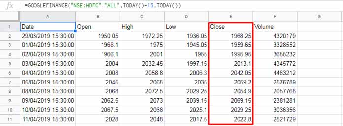
See the below example screenshot. In that, I have marked column 5. How to find the max/min values in that column?

Changes in Formulas:

1. In Query, you just need to change column number to 5 in the Max aggregation function and in the labeling.
2. Regarding the DMAX or DMIN, change the field number to 5.
3. In the Min/Max Index combo, change the offset number to 5. How?.

Query:

=QUERY(GOOGLEFINANCE("NSE:HDFC","ALL",TODAY()-15,TODAY()),"Select Max(Col5) label Max(Col5)''",1)

Changes: “Col2” to “Col5”.

DMAX:

=DMAX(GOOGLEFINANCE("NSE:HDFC","ALL",TODAY()-15,TODAY()),5,{"Date";">"&text("30/12/1899","dd/mm/yyyy")})

Changes: Field number 2 to 5.

MIN/Index:

=MAX(index(GOOGLEFINANCE("NSE:HDFC","ALL",TODAY()-15,TODAY()),0,5))

Changes: Offset column 2 to 5.

This way you can find the Min values too from a multi-column GoogleFinance historical data. For that just change Max to Min.

Additional Resources:

1. How to Find Max Value in Each Row in Google Sheets [Array Formula].
2. Vlookup to Only Return Values from Max Rows in Google Sheets.
3. How to Exclude 0 From MIN Function Result in Google Sheets.
4. Sum Large/Max n Values Based on Criteria in Google Sheets.
5. Find Max N Values in a Row and Return Headers in Google Sheets.