How to Find Max Value in Each Row in Google Sheets

To find the maximum value in each row in Google Sheets, you can use three main formula options: the MAX function with BYROW, a DMAX-based formula, and a QUERY-based formula.

Before the introduction of the BYROW function (a Lambda helper function), the QUERY and DMAX methods were the primary options. I’ll share all three options with you, but the MAX and BYROW combination is the simplest and most efficient. So, let’s start with that.

For this example, we’ll use the sample data in A1:F10, and the range we want to evaluate for maximum values is B2:F10.

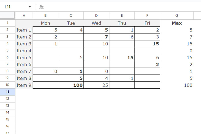
Sample data for finding the maximum value in each row

MAX and BYROW Combo for Getting Max Value in Each Row

To get the maximum value in each row, you can use the following simple, non-array formula in cell G2 and drag it down to G10:

=MAX(B2:F2)

However, we can convert this into an array formula to avoid dragging the formula manually.

Steps to Convert It Into an Array Formula:

First, create a custom LAMBDA function:
LAMBDA(row, MAX(row))
Next, apply this LAMBDA function to each row using the BYROW function:
=BYROW(B2:F10, LAMBDA(row, MAX(row)))

This formula in cell G2 will return the row-wise maximum value for each row in the specified range. This method is the simplest and most efficient way to find the max value in each row in Google Sheets.

QUERY-Based Formula for Getting Max Value in Each Row

Another option is to use the QUERY function. However, by default, QUERY returns the maximum values for each column, not each row. To get the max values for rows, we need to transpose the data.

Here’s the formula to get the max values for each row:

Transpose the data and apply QUERY:
=INDEX(TRANSPOSE(QUERY(TRANSPOSE(B2:F10), "SELECT MAX(Col1), MAX(Col2), MAX(Col3), MAX(Col4), MAX(Col5), MAX(Col6), MAX(Col7), MAX(Col8), MAX(Col9)", 0)), 0, 2)
The INDEX function is used here to remove the label column returned by the QUERY.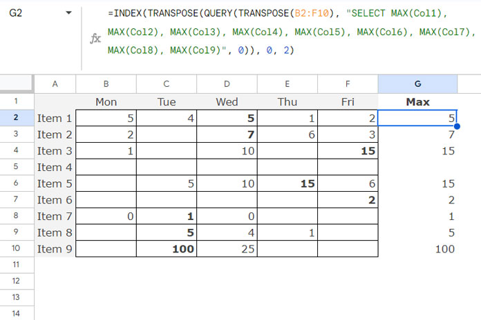
To avoid hardcoding the column names (MAX(Col1), MAX(Col2)…), we can dynamically generate this part using SEQUENCE, COLUMNS, and TEXTJOIN:
=ArrayFormula(TEXTJOIN("),", TRUE, "MAX(Col"&SEQUENCE(COLUMNS(TRANSPOSE(B2:F10))))&")")
Final dynamic QUERY formula:
=INDEX(TRANSPOSE(QUERY(TRANSPOSE(B2:F10), "Select "&TEXTJOIN("),", TRUE, "MAX(Col"&SEQUENCE(COLUMNS(TRANSPOSE(B2:F10))))&")")), 0, 2)

This method is a bit more complex than the BYROW method but works efficiently, especially when using dynamic ranges.

DMAX-Based Formula for Getting Max Value in Each Row

Before the introduction of the BYROW function, another method to find the max value in each row was using the DMAX function. However, like QUERY, DMAX is designed to return the max value from columns rather than rows.

To use DMAX for rows, we need to transpose the data and add a structured header.

Syntax:

DMAX(TRANSPOSE(database), field, criteria)

Steps to Use DMAX for Max Value in Each Row:

Add a header row by stacking row numbers to act as the new “header”:
=HSTACK(ROW(B2:B10), B2:F10)
Transpose the data to structure it properly for the DMAX function:
TRANSPOSE(HSTACK(ROW(B2:B10), B2:F10))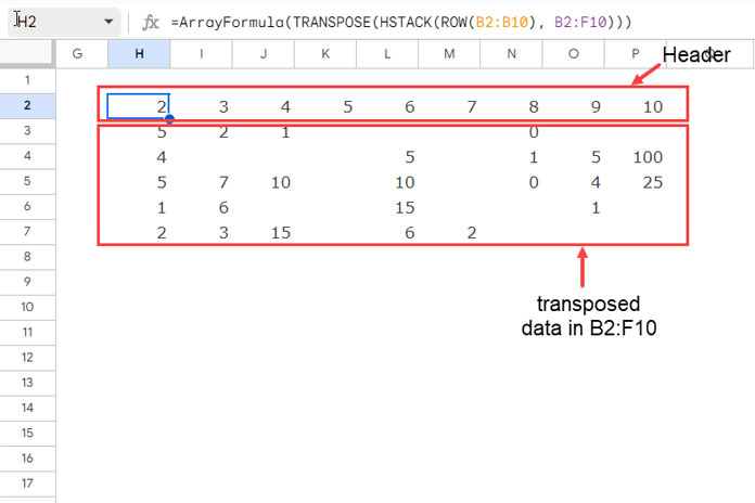
Use this transposed data as the database for the DMAX function. Here is the final formula:

=ArrayFormula(
   DMAX(
      TRANSPOSE(HSTACK(ROW(B2:B10), B2:F10)), 
      SEQUENCE(ROWS(B2:B10)), 
      {IF(,,); IF(,,)}
   )
)

In this formula, SEQUENCE(ROWS(B2:B10)) dynamically returns the column index (field) for the output, and {IF(,,); IF(,,)} serves as an empty criteria range.

This formula will return the maximum values for each row, but it’s more complex and less intuitive compared to the BYROW function.

Conclusion

Of the three methods, which one is best for finding the max value in each row in Google Sheets?

I would recommend the MAX and BYROW combination. It’s straightforward and works efficiently in most cases. However, if you are dealing with very large datasets and the BYROW formula runs into performance issues, you might consider using the DMAX method for better efficiency.

Resources

24 COMMENTS

John Usher June 5, 2021 At 4:05 pm

Gosh! Thank you so much. It’s elegant.

John Usher May 27, 2021 At 9:54 pm

Hi Guys,

I need help…

I have 5 columns in google sheets – example column 1 – “visual”, column 2 – “auditory”, column 3 – “kinaesthetic”, column 4 – “taste”, column 5 – “smell”.

I want to add a formula in column 6 to find the highest value in the row for these five columns, but I want it to return the column name.

Any help, comments, or formulas would be of great help.

Thanks

- Prashanth May 28, 2021 At 10:51 am
  
  Hi, John Usher,
  
  I indeed have a solution already posted that also includes a sample sheet. You can find that here – Column Header of Max Value in Google Sheets Using Array Formula.
  
  It has a drawback! If there are multiple max values, you won’t get the column header of both.
  
  If you want help implementing the above-mentioned solution, please leave your Sheet link in your reply (I won’t publish that comment).
  
- Prashanth May 29, 2021 At 11:02 am
  
  Hi, John Usher,
  
  Here I recommend a non-array formula. In BF2 insert the below Filter and drag-down.
  
  =textjoin(", ",true,filter($AZ$1:$BD$1,AZ2:BD2=max(AZ2:BD2)))
  
lightmare February 7, 2021 At 11:39 pm

Hi, I think I’ve found a better method of doing this.

Since I wasn’t able to use your method because I had too many rows (exceeding TEXTJOIN length limit), I wrote a function RowWiseMax() in JavaScript and used that. But then I figured out another way to do row-wise max using just the built-in functions, which works with thousands of rows.
Here it is:
=ARRAYFORMULA(DMAX(TRANSPOSE(A3:G6), SEQUENCE(ROWS(A3:G6)), {IF(,,);IF(,,)}))

- Prashanth February 8, 2021 At 11:06 am
  
  Hi, lightmare,
  
  Very interesting. If possible share it with other readers. You can share the sheet via comment. If working properly, I may copy your sheet, add due credit to you, and will publish the sheet in Copy mode.
  
  - lightmare February 14, 2021 At 6:49 am
    
    Hi, sorry I forgot to link the example doc I tested this with, here it is:
    
    https://docs.google.com/spreadsheets/d/1x2q5ByM-BUkMiI791N77pFmNpo33IRPks7ElqbikOdQ/copy
    
    - Prashanth February 14, 2021 At 11:51 am
      
      Hi, lightmare,
      
      Thanks for sharing the sheet. I have copied it and the copied sheet link included in your comment to avoid future SEO issues due to file deletion.
      
      Thanks again.
      
    - Aurelien Begot November 29, 2021 At 4:15 am
      
      This is AWESOME
      
- Prashanth February 8, 2021 At 2:43 pm
  
  Hi, lightmare,
  
  I could manage to write a DMAX formula based on your input. In that, the Transpose and Sequence come into use. But I didn’t use the IF.
  
  That means the syntax may not be the same as yours.
  
  I’ll write the formula example soon and of course, give you the due credit.
  
  Thanks for enlightening me.
  
- Prashanth February 13, 2021 At 3:26 pm
  
  Hi, lightmare,
  
  Here is the said tutorial.
  
  Row-Wise MIN Using DMIN in Google Sheets.
  
  Thanks.
  
  - lightmare February 14, 2021 At 7:01 am
    
    Hi, thank you for the detailed guide, and sorry for not helping you out with it. I drifted away to other tasks and didn’t check back here in a while.
    
    In my original post, I explained each part of the formula, including the strange use of IF. No idea why the post was cut short, there was no indication of a comment length limit.
    
    I see in your guide you replaced the IF(,,) hack with essentially filtering on identity; that’s clever, why hadn’t I thought of that? 😀
    
    - Prashanth February 14, 2021 At 11:55 am
      
      Thanks.
      
- Jorge Eduardo February 14, 2023 At 11:30 pm
  
  Wow, thanks, Lightmare. I’ve been looking for this solution since a long time ago. I can now clean several tables. Thanks to this.
  
Edgar December 18, 2019 At 11:50 am

Any chance to have something for a minIF case?

Austria August 20, 2019 At 1:51 pm

Good day,

What if I want to see two values,

The highest value and the second to the highest values per row.

- Prashanth August 20, 2019 At 5:56 pm
  
  Hi, Austria,
  
  Right now, I don’t have an array formula for that. Here is a non-array formula.
  
  Assume the values are in B3:G.
  
  Enter this formula in cell H3 and copy/drag down.
  
  =ArrayFormula(large(B3:G3,{1,2}))
  
  Best,
  
  - DNel February 16, 2021 At 10:29 am
    
    Any further luck with this?
    
    - Prashanth February 16, 2021 At 12:28 pm
      
      Hi, DNel,
      
      I do have the solution now. I will explain the same in my coming tutorial.
      
      You will get the link below soon!
      
    - Prashanth February 16, 2021 At 6:47 pm
      
      Hi, Dnel,
      
      Here is the tutorial link.
      
      Return First and Second Highest Values in Each Row in Google Sheets.
      
E Kain December 20, 2018 At 9:58 am

The formulas in the above article are quite brilliant! While I already knew how those individual functions work in GSheets, the clever way shown here of combining them together was eye-opening.
However, I was stymied by Google’s column limit when I tried to use it on a dataset that was 7000+ rows long.
A simpler workaround I discovered was as follows (assume in this example that the top row is header):

=ArrayFormula(if(GTE(A2:A,B2:B),A2:A,B2:B))

While MAX doesn’t play nice with array formulas, I haven’t had trouble with many of the other comparators, and since the GTE function returns “TRUE” if the first term is >= the second term, a simple “if” statement seems to do the trick. Also, it seems to have the same ability of not requiring a defined “end” to the dataset, and seems to work fine on both short or long spreadsheets without worrying about where the last row is found.

Please beware that I have not rigorously tested this—I’ve only used it for my specific needs on a spreadsheet for work. Therefore, if someone out there sees a flaw with this, please let me know so I can save myself a headache down the road! 🙂

- Prashanth December 20, 2018 At 10:19 am
  
  Hi, E Kain,
  
  Thanks for sharing the tip!
  
  I’ll definitely test it and update you.
  
  Cheers!
  
- Prashanth December 22, 2018 At 10:38 am
  
  Hi, E Kain,
  
  Today I got time and checked your formula. Of course, it works! But assume you have 20 columns. Then the formula would be very complex and difficult code without error.
  
  My formula works well! But when there are a large number of rows, it fails miserably due to the limitation of Join/Textjoin functions.
  
  Thanks.
  
- Flemming Steffensen November 13, 2019 At 5:50 pm
  
  I know this is an old thread, but just for others to understand the complexity expansion of E Kain’s proposal, I wanted to show this example:
  
  With two columns (as suggested), the formula is seemingly simple:
  
  =ArrayFormula(if(GTE(D97:D99,E97:E99),D97:D99,E97:E99))
  
  But already at three columns, the formula becomes hard to read (and especially maintain):
  =ArrayFormula(if(GTE(if(GTE(D93:D95,E93:E95),D93:D95,E93:E95), if(GTE(E93:E95,F93:F95),E93:E95,F93:F95)),if(GTE(D93:D95,E93:E95),D93:D95,E93:E95), if(GTE(E93:E95,F93:F95),E93:E95,F93:F95)))