First and Second Highest Values in Each Row in Google Sheets

With the help of the BYROW and LARGE functions, you can easily find the first, second, or nth highest value in each row in Google Sheets.

Table of Contents

Sample Data

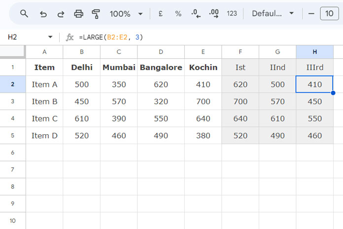
Assume you have item descriptions in one column and sales from different regions in the adjacent columns. You can then find each item’s first, second, and third highest sales across these regions. Below is an example of how your data might look:

Item	Delhi	Mumbai	Bangalore	Kochin
Item A	500	350	620	410
Item B	450	570	320	700
Item C	610	390	550	640
Item D	520	460	490	380

The above data is in the range A1:E5. Let’s find the first, second, and third highest values in each row and display them in F2:F5, G2:G5, and H2:H5, respectively.

First, second, and third highest values in each row of a Google Sheets table

Regular Non-Array Solutions

Finding the First Highest Value:

To find the first highest value for each row, enter the following LARGE formula in cell F2 and drag the fill handle down:

=LARGE(B2:E2, 1)

Finding the Second Highest Value:

To get the second highest value, replace 1 with 2 in the formula, and then drag it down:

=LARGE(B2:E2, 2)

Finding the Third Highest Value:

For the third highest value, replace 1 with 3 in the formula and drag it down:

=LARGE(B2:E2, 3)

Array Formula to Find the First, Second, and Third Highest Values in Each Row

When you want to consider a row, rather than a single cell, as a single entity and apply a LAMBDA function to each row, you can use the BYROW function.

The syntax is:

BYROW(array_or_range, lambda)

In this case, the array or range is B2:E5. Let’s write the LAMBDA function to apply to each row.

Finding the First Largest Value

We will start by coding the formula to find the first largest value in each row. For this, we will use the following LARGE formula, which we used earlier in cell F2:

=LARGE(B2:E2, 1)

We can convert this to a LAMBDA function, which follows the syntax:

LAMBDA([name, …], formula_expression)

In the LARGE formula, replace B2:E2 with a meaningful name, such as row, and define that in LAMBDA as follows:

LAMBDA(row, LARGE(row, 1))

The LAMBDA function to find the first largest value in each row is now ready. Simply use this within the BYROW function as follows:

=BYROW(B2:E5, LAMBDA(row, LARGE(row, 1)))

Clear any values in F2:F5 and enter this formula in F2 to get the first largest value in each row.

Finding the Second and Third Largest Values

To get the second, third, or nth largest value in each row, replace 1 with n, such as 2, 3, etc. For example:

For the second largest value:
=BYROW(B2:E5, LAMBDA(row, LARGE(row, 2)))
For the third largest value:
=BYROW(B2:E5, LAMBDA(row, LARGE(row, 3)))