I have array and non-array solutions to get min dates that ignore blanks in each row in Google Sheets. That includes Lambda formulas too.
Ignoring blanks is very important in this context. Do you know why?
Assume you have a date range of B2:F7.
You want to get min dates ignoring blanks in each row in this range.
There is no issue getting the correct min date from this range;
- If there is at least one date in each row.
- The range does not contain any values other than dates.
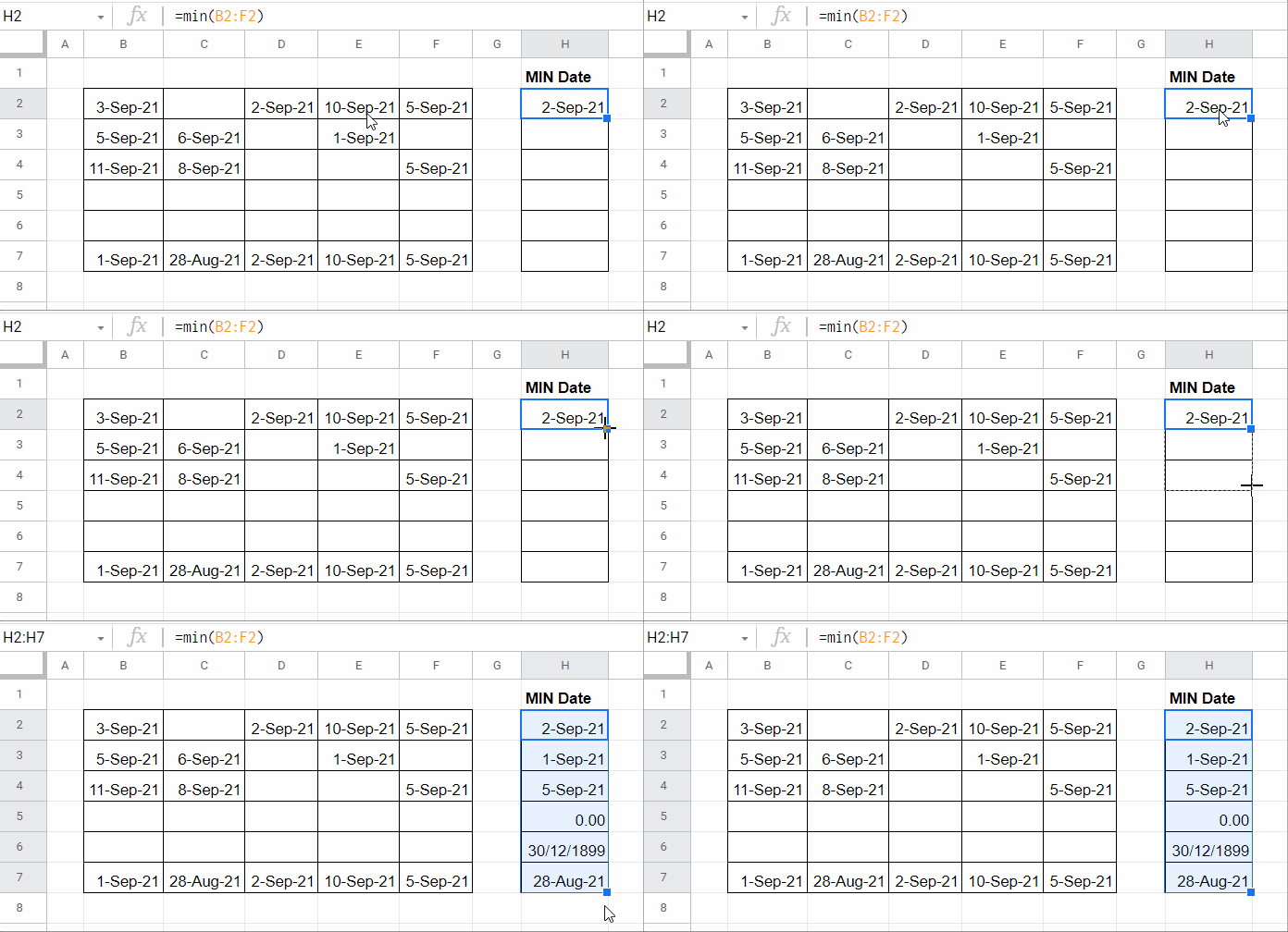
You can use the below MIN formula for that in cell H2 and copy-paste it down.
A] MIN Non-Array Formula:
=min(B2:F2)You can also use a DMIN-based array formula for that.
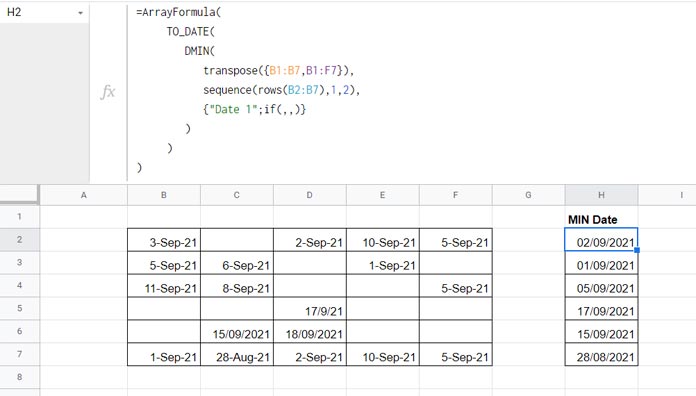
B.1] DMIN Array Formula (Empty H2:H7 and then insert it in H2 alone):
=ArrayFormula(
     TO_DATE(
        DMIN(
           transpose({B1:B7,B1:F7}),
           sequence(rows(B2:B7),1,2),
           {"Date 1";if(,,)}
        )
     )
)
If you want to learn the above DMIN array formula, please read my guide – Row-Wise MIN Using DMIN in Google Sheets.
But please note that the above formula is slightly different from the formula explained in the linked tutorial.
Here I have brought some performance enhancements which are self-explanatory.
Instead of the above DMIN, we can now expand the MIN using the BYROW Lambda helper function.
B.2] MIN Lambda Array Formula (Empty H2:H7 and then insert it in H2 alone): New!
=byrow(H2:H7,lambda(r,min(r)))What Happens When Blank Rows Are Present between Date Rows?
You won’t get blank in the corresponding result cell if any row is blank.
Instead, when using MIN (A or B.1 formula), you will get 0 or 30/12/1899 depending on the result cell formatting.
When Using DMIN, you will get 30/12/1899, irrespective of the formatting.
So you won’t be able to use the above formulas for getting the min dates ignoring blanks in each row in Google Sheets.
Let’s test it by following the below steps.
- Empty the range B5:F6.
- Select B5:F5 and go to the menu Format > Number > Number.
- Select B6:F6 and go to the menu Format > Number > Date.
We have formatted two rows differently.
Insert the above Min formula in cell H2 and copy it down and see the bizarre output.

Also, try the above DMIN.
Formulas to Get Min Date Ignoring Blanks in Each Row
Non-Array Solution
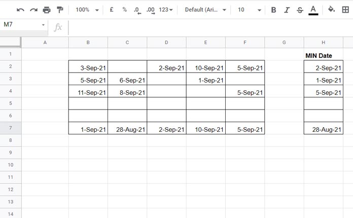
C] If you prefer a non-array solution, use the FILTER function to filter out blank cells in rows and use MIN.
=iferror(min(filter(B2:F2,datevalue(B2:F2))))Select the outputs and format the date values to dates.
Array Formulas to Get Min Date Ignoring Blanks in Each Row
Here are the array formulas to get the min date, ignoring blanks in each row in Google Sheets.
Generic Formula: IF(DMIN_Array_Formula >0, DMIN_Array_Formula,)
D] DMIN Formula:
=ArrayFormula(
     TO_DATE(
        if(
           DMIN(
              transpose({B1:B,B1:F}),
              sequence(rows(B2:B),1,2),
             {"Date 1";if(,,)}
           )>0,
           DMIN(
              transpose({B1:B,B1:F}),
              sequence(rows(B2:B),1,2),
              {"Date 1";if(,,)}
           ),
        )
     )
)
Output:

Since the formula is capable of ignoring blank cells between dates, I have opened the range.
I mean, replaced B7 and F7 with B and F, respectively.
What about a Lambda alternative?
E] Lambda Formula: New!
=byrow(B2:F,lambda(r, to_date(iferror(min(filter(r,datevalue(r)))))))Impact of Zero Values
I won’t expect a user would enter 0 between dates instead of leaving cells blank.
But it may happen when he has imported data processed within Sheets.
In such scenarios, there won’t be an issue if you use formulas C or E.
I mean with the MIN-based array and non-array formulas we have used above to get the min / smallest date ignoring blanks in each row.
Regarding formula D, the complex-looking array formula, you should replace B1:F (appears twice) with the below formula part.
iferror(datevalue(B1:F))That’s all. Thanks for the stay. Enjoy!
Resources:
- How to Exclude 0 From MIN Function Result in Google Sheets.
- Return Blank Instead of 30-12-1899 in Google Sheets Formulas.
- Highlight Min Excluding Zero and Blank Cell in Google Sheets.
- Finding Max and Min Values in GoogleFinance Historical Data in Sheets.
- Min in Vlookup in Google Sheets – Formula Examples.
- Hyperlink Max and Min Values in Column or Row in Google Sheets.
- How to Retrieve Column Header of Min Value in Google Sheets.


