Google Sheets has abundant formula options for retrieving the column header of a min value in a row.
In this post, you will get three of the best formulas; a non-array formula (Filter) and two array formulas (Vlookup and Lambda). They work quite differently.
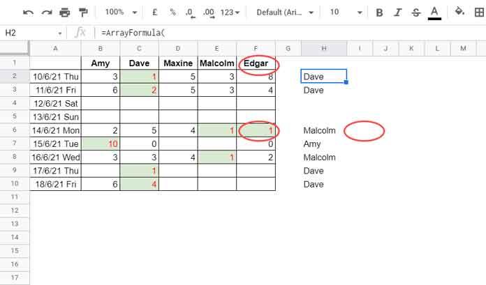
If there is more than one min value in a row, the non-array formula (Filter) and one of the array formulas (Lambda) will return multiple column headers.
At the same time, the other array formula (Vlookup) will only return the first column header.
The advantage of the array formulas is they would return the min value header(s) in every row.
Please note that here column header means field label in the topmost row of your table.
Formula to Return the Column Header of Min Value in Google Sheets
Assume five employees are working under you. You want to assess their daily sales and find who is underperforming each day.
Here is the sample data in hand.
You can find the employee names on the column header (header row) and their date-wise sales in corresponding columns.
| Amy | Dave | Maxine | Malcolm | Edgar | |
| 10/6/21 Thu | 3 | 1 | 5 | 3 | 8 |
| 11/6/21 Fri | 6 | 2 | 5 | 3 | 4 |
| 12/6/21 Sat | |||||
| 13/6/21 Sun | |||||
| 14/6/21 Mon | 2 | 5 | 4 | 1 | 1 |
| 15/6/21 Tue | 10 | 0 | |||
| 16/6/21 Wed | 3 | 3 | 4 | 1 | 2 |
| 17/6/21 Thu | 1 | ||||
| 18/6/21 Fri | 6 | 4 |
We can use QUERY or SORTN functions for this purpose. But I would prefer Filter here.
Assume the above table is in the range A1:F10.
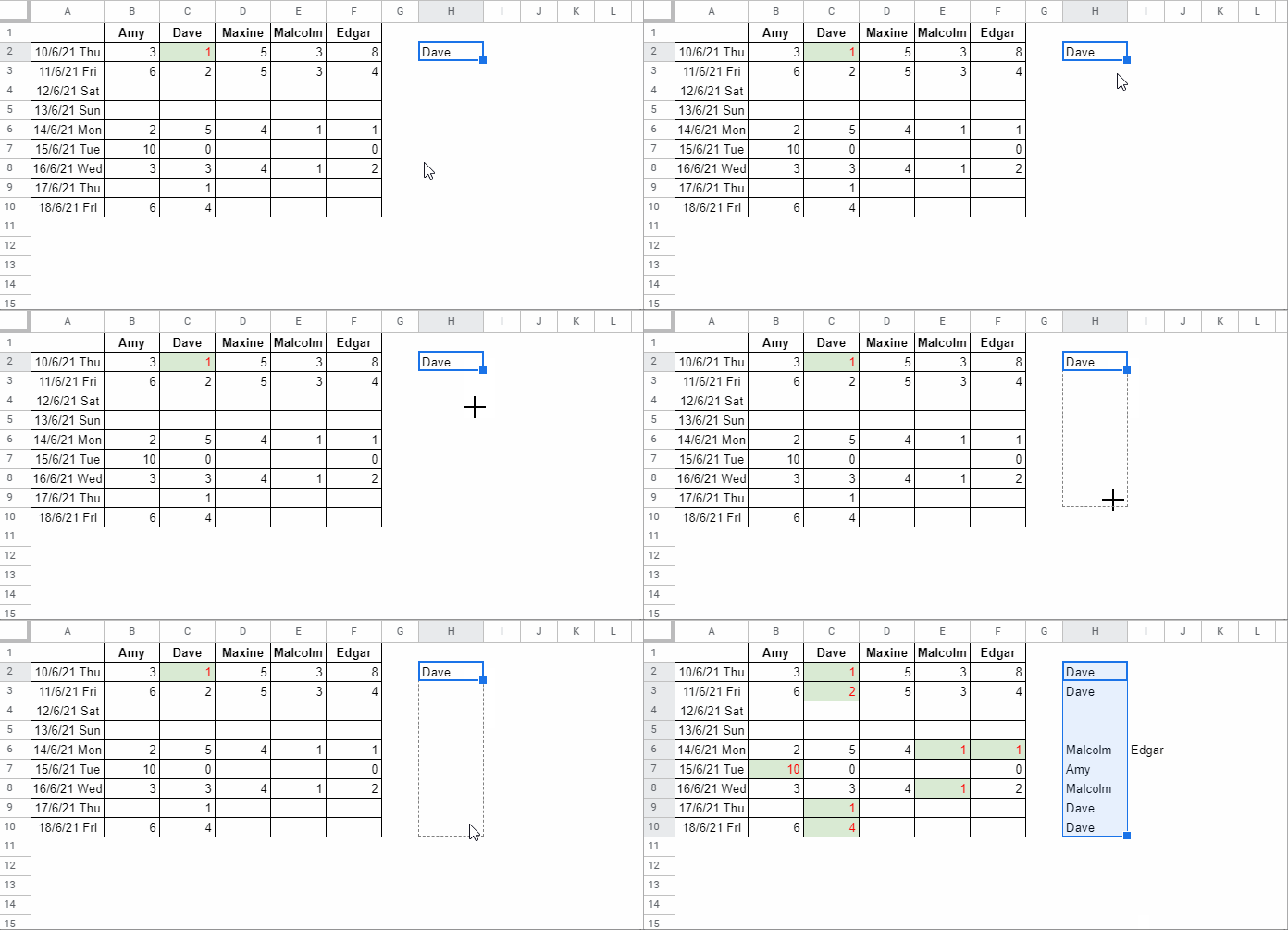
Then we can use the below Filter formula in cell H2. Drag it down until cell H10 to get the column header of the min value in every row.
=ifna(
     filter(
        $B$1:$F$1,
        B2:F2=minifs(B2:F2,B2:F2,">0"),
        B2:F2<>""
     )
)
Can you please explain this Google Sheets formula?
Yep! Here you go!
- The MINIFS returns the min value of the sales quantity in B2:F2, excluding zero and blanks.
- The FILTER formula filters the min value headers (employee names) matching the MINIFS result.
- In a blank row or a row that only contains 0, the MINIFS will return 0. The second condition in FILTER, i.e.,
B2:F2<>"", is to return #N/A in that case. - The IFNA removes the above error.
- When you drag the formula down, it applies to other rows.
See this example live (GIF).

If you are a Google Sheets enthusiast, you might want to know the ‘rule’ I have used to format the range B2:F10. Here it is.
=and(len($H2),$B2:$F2=minifs($B2:$F2,$B2:$F2,">0"))You can use this rule in Format > Conditional formatting.
Array Formula 1 to Retrieve the Column Header of Min Value – VLOOKUP
We can use a Vlookup array formula to retrieve the column header of the min values in Google Sheets. There is a better Lambda option now. We will try that later.
It has a drawback. In the above example, the filter formula returns the names “Malcolm” and “Edgar” in row # 6 as the min value, i.e., 1, repeats twice.
My following array formula would only return the first min header, i.e., “Malcolm.”
=ArrayFormula(
     ifna(
        if(len(A2:A),
           vlookup(
              row(A2:A)&"~"&
              dmin(
                 transpose(if(A2:F>0,A2:F,)),
                 sequence(rows(A2:A),1),
                 {if(,,);if(,,)}
              ),
              Query(split(flatten(row(A2:A)&"~"&if(B2:F>0,B2:F,)&"🐟"&B1:F1),"🐟"),
              "Select * where Col1 is not null and Col2 is not null")
              ,2,0
          ),
        )
     )
 )
If you prefer to use this array formula to retrieve the column header of the min value in each row in Google Sheets, you may want to go through the formula explanation.
Note:- If multiple min values exist in a row, the array formula would only return the min header of the first occurrence from left to right.
Formula Explanation
Generic Formula: vlookup(row_nos&min_each_row,unpivot_table,2,0)
Vlookup Syntax: VLOOKUP(search_key, range, index, [is_sorted])
We have used VLOOKUP to retrieve the column header of the min value, excluding 0, in each row. Here are the expressions/references used in the arguments.
SEARCH_KEY: row_nos&min_each_row
RANGE: unpivot_table
INDEX: 2
IS_SORTED: 0
I know I must explain the search key and range in Vlookpup for you to understand how it works.
SEARCH_KEY
The search key here is the combination of min and row numbers (row_nos&min_each_row) in each row. Here is that portion of the formula.
row(A2:A10)&"~"&
dmin(
     transpose(if(A2:F10>0,A2:F10,)),
     sequence(rows(A2:A10),1),
     {if(,,);if(,,)}
)
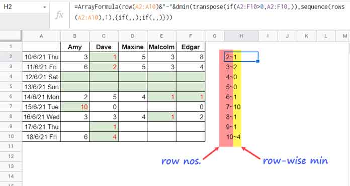
It will return the following result if you use it as an ArrayFormula.

In this part of the formula, I have used DMIN as per the logic detailed here – Row-Wise MIN Using DMIN in Google Sheets.
RANGE
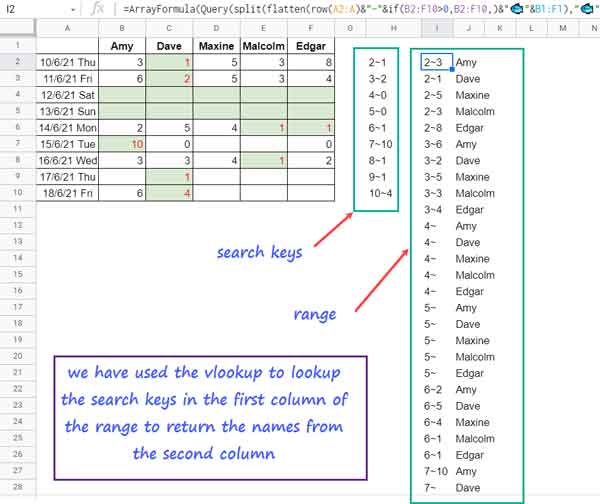
The range is the unpivot B1:F10 data. When doing so, the row numbers from A2:A10 are combined with the values (sales quantities) in B2:F10.
Here is the relevant part from the formula (the ranges are closed here from A2:A and B2:B to A2:A10 and B2:B10). The FLATTEN function with SPLIT does the job.
Query(split(flatten(row(A2:A10)&"~"&if(B2:F10>0,B2:F10,)&"🐟"&B1:F1),"🐟"),
"Select * where Col1 is not null and Col2 is not null")
It will work with the array formula as a standalone in Sheets. Here is that output.

Related: A Simple Formula to Unpivot a Dataset in Google Sheets.
Array Formula 2 to Retrieve the Column Header of Min Value – LAMBDA
Google Sheets has now the capability to expand non-array formulas to each row. This is possible using LAMBDA helper functions (LHF).
We will use BYROW LHF to expand our first filter-based non-array formula. That way, we can get the column header of the min value in each row in Google Sheets.
=byrow(B2:F,lambda(r, join(", ",ifna(filter($B$1:$F$1,r=minifs(r,r,">0"),r<>"")))))The formula combines column names (headers) if there are multiple occurrences of min values (e.g., row # 6).
So unlike the non-array formula, which returns “Malcolm” and “Edgar” in two cells (row #6), here the Lambda formula will JOIN them.
That’s all. Thanks for the stay. Enjoy!
Related: Column Header of Max Value in Google Sheets Using Array Formula.


