When you have multiple columns of data with numbers below, you might want to find the column header of the max value in each row in Google Sheets.

For example, suppose you have items listed in column A and their stock quantities across three warehouses in the next three columns. In this case, you may want to retrieve the warehouse name for each item with the highest quantity.

This involves finding the maximum value and then locating the corresponding header. This process should repeat for each row to cover all items. Sometimes, there may be a tie, in which case multiple headers should be returned.

We can use either array formulas or non-array formulas to find the column header of the max value in Google Sheets. Let’s explore the examples.

Example: Finding the Column Header of the Max Value in Google Sheets

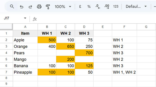
In the following dataset, column A contains item names, while columns B, C, and D hold the quantities for Warehouse 1, Warehouse 2, and Warehouse 3.

To find the column header of the max value for the first item, use the following formula in cell F2:

=TEXTJOIN(", ", TRUE, IFNA(FILTER($B$1:$D$1, XMATCH(IF(B2:D2="", NA(), B2:D2), MAX(B2:D2)))))

Drag this formula down to apply it to all rows.

• If there are multiple matching values, the corresponding headers will be returned as a comma-separated list.

Formula Explanation

The formula filters the range $B$1:$D$1 based on the condition below:

XMATCH(IF(B2:D2="", NA(), B2:D2), MAX(B2:D2))

Where:

• XMATCH(IF(B2:D2="", NA(), B2:D2), MAX(B2:D2)) – Matches each value in the row against the max value and returns its position or #N/A if not found. For example, if the maximum value is in the first column, it returns {1, #N/A, #N/A}.
  • IF(B2:D2="", NA(), B2:D2) – Converts empty cells into #N/A errors and keeps values in other cells. This ensures that blank cells are not considered when finding the max value.
  • MAX(B2:D2) – Returns the highest value in the row.
• FILTER($B$1:$D$1, condition) – Filters the header row (B1:D1) based on the condition (XMATCH result). If the condition is a number (not an error), the corresponding header is returned.
• TEXTJOIN(", ", TRUE, IFNA(...)) – Joins multiple headers (if any) into a single cell.

Since the header row reference ($B$1:$D$1) is absolute, it remains unchanged when dragging the formula down, while the row conditions update dynamically.

This is how the formula identifies the column header of the maximum value in each row.

Array Formula to Find the Column Header of the Max Value in Each Row

Drag-down formulas have limitations. For instance, you’ll need to copy the formula to new or inserted rows unless you’re using structured tables. To avoid this, you can convert the formula into an array formula using the BYROW and LAMBDA functions:

=BYROW(B2:D9, LAMBDA(r_, TEXTJOIN(", ", TRUE, IFNA(FILTER(B1:D1, XMATCH(IF(r_="", NA(), r_), MAX(r_)))))))

This formula converts the previous logic into a custom unnamed LAMBDA function, where:

• r_ represents the current row.
• BYROW applies the formula to each row in the array, returning the column header of the max value for each row.

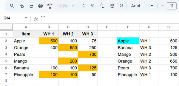
Additional Tip: Creating a Table with Items, Max Values, and Headers

If you want to see the max value and corresponding headers for all items in one table, use this approach:

=LET(
   data, ARRAYFORMULA(SPLIT(FLATTEN(A2:A&"|"&B1:D1&"|"&B2:D), "|")), 
   ftr, FILTER(data, CHOOSECOLS(data, 3)>0), 
   SORTN(SORT(ftr, 1, 1, 3, 0), 9^9, 2, 1, 1)
)

Where:

• A2:A contains the items.
• B1:D1 holds the headers.
• B2:D holds the values.

Pros and Cons:

Pros:

• Doesn’t rely on LAMBDA, making it resource-friendly.
• Returns headers of max values for all items at once.

Cons:

• If there are multiple max values for an item, it only returns one header, not all.

Explanation of the Formula

• ARRAYFORMULA(SPLIT(FLATTEN(A2:A&"|"&B1:D1&"|"&B2:D), "|")) – Converts the data into a flattened, unpivoted format (named data).
• FILTER(data, CHOOSECOLS(data, 3)>0) – Filters out blank rows from the data to improve performance (named ftr).
• SORTN(SORT(ftr, 1, 1, 3, 0), 9^9, 2, 1, 1) – Sorts the filtered (ftr) items alphabetically, then by max quantity in descending order, ensuring the max value is at the top. SORTN removes duplicates, leaving unique items with their max value and header.

Sample Sheet

Sample Sheet

Resources

• Find Max N Values in a Row and Return Headers in Google Sheets
• Lookup and Retrieve Column Headers in Google Sheets
• Search Across Columns and Return the Header in Google Sheets
• How to Retrieve Column Header of Min Value in Google Sheets
• Get the Headers of the First Non-Blank Cell in Each Row in Google Sheets
• Get the Header of the Last Non-Blank Cell in a Row in Google Sheets