We can use the database function DMIN to return row-wise min in Google Sheets. I’m sure it’s an unfamiliar formula to many of you.
In this post, I am going to follow the syntax suggested by one of my readers “Lightmare” (user name) to return the min in each row in Google Sheets.
I wish to link to his comment, but could not find a way to do so. You can read his comment under my post – How to Find Max Value in Each Row in Google Sheets [Array Formula].
His idea was about max value using DMAX. The same applies to the min value using DMIN.
So I am writing the DMIN formula. You can replace DMIN with DMAX to change the min value to the max value.
The formula will reside within the very first row and will return the min value in each row in Google Sheets.
That means we will use a DMIN based array formula for the same.
I have already a formula to return the min value in each row (row-wise min) in Google Sheets. You can read that here – How to Use MIN in Array in Google Sheets for Expanded Results.
But it has one issue 🙁
What’s that?
In the said formula I have used the JOIN function which has a limitation. It will possibly work in a limited number of rows. It’s the case with the alternative function TEXTJOIN.
From my test, the row-wise min in Google Sheets using the DMIN function has the advantage of working with a very large data set.
It may slow down the performance of your sheet. But will work.
Let’s see how to use the DMIN database function to return row-wise min value in Google Sheets.
Before proceeding, only keep the required number of columns and rows in your sheet. That will help the formula to work in a better way.
Return Row Wise MIN Using DMIN in Google Sheets
First of all, as usual, we need a sample sheet to proceed further.
I have the following data (range A1:E1000). The DMIN formula in cell F1 returns the min value in each row in that column.
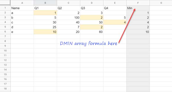
I have included my sample sheet with the formula for your convenience. You can find the link at the end of this tutorial.
Here is the formula in cell F1.
={"Min";ArrayFormula(if(len(A2:A),(DMIN(transpose({{"Row";sequence(rows(A2:A1000),1)},B1:E1000}),sequence(1000,1,2),transpose({"Row",B1:E1}))),))}Let’s see how this DMIN array formula works for every row from a single cell. Find the logic and formula explanations below.
What Are the Changes Required in a Different Table?
The above formula is written for a total of 1000 rows. Change it to the number of rows you require.
There are some changes that you should make to this formula to adapt to a new table. Here are them.
1. The range B1:E1000 is the numeric column range from which I wish to return the row-wise min values using the DMIN. So change it as per the numeric columns in your range.
2. The range B1:E1 should contain the title as we are dealing with a database function.
If your numeric columns are in a different range, not B1:E1000, accordingly change B1:E1.
3. The formula part rows(A2:A1000) is just to return the total number of rows in your sheet except for the header. So there won’t be any changes in this unless your table is starting from a different row.
I mean if your table is starting from row # 10 and in which the first row contains the headers and from row 11 onwards the numbers, then replace rows(A2:A1000) to rows(A11:A1000).
4. Similarly, len(A2:A1000) must be changed to len(A11:A1000). Unlike the above in point # 3, here you may require to change the column reference with the first column in your table.
The above are the changes that you may require to make in the DMIN formula to return row-wise min in for your table in Google Sheets.
Let’s now go to the formula Explanation.
DMIN Array Formula for Row-Wise MIN in Google Sheets – Logic
We can use the DMIN function to return the MIN value in a single column or multiple columns. That’s the logic of the above row-wise min formula.
Let’s consider the same sample data above.
To return the min value in column B (Q1), we can use the following DMIN formula.
=dmin(A1:E6,B1,A1:A6)Or;
=dmin(A1:E6,2,A1:A6)For returning the min in every column, we can use the same formula as an Array Formula below.
=ArrayFormula(dmin(A1:E6,B1:E1,A1:A6))Or;
=ArrayFormula(dmin(A1:E6,{2,3,4,5},A1:A6))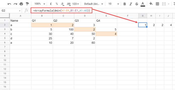
Here I am going to reveal an important step that I will use in row-wise MIN using DMIN in Google Sheets.
To return the min value in every row, let’s transpose the data and apply the above formula. So the result will be row-wise min.
But when transposing, we should make some changes as DMIN is a database function. It heavily depends on the header row (fields) in the calculation.
So we may require to use some workarounds. Here are them.
I’ll explain the formula for the range A1:E6 (limited range). So that you can easily understand and test it in your sheet.
Later change it to A1:E1000 as per my master DMIN row-wise min formula.
Row-Wise MIN Explained for Limited Range
Formula:
=ArrayFormula(DMIN(transpose({{"Row";sequence(rows(A2:A6),1)},B1:E6}),sequence(5,1,2),transpose({"Row",B1:E1})))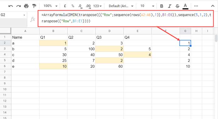
Formula Explanation:
Syntax: DMIN(database, field, criteria)
We have used the below expressions in each argument.
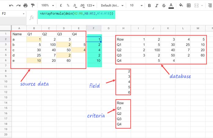
database: transpose({{"Row";sequence(rows(A2:A6),1)},B1:E6})
It makes the sample data looks like as below.
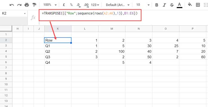
Before transposing, the formula first replaces A1:A6 with row numbers {"Row";sequence(rows(A2:A6),1)} and combine the rest of the range B1:E6 with it.
When we transpose it, we will get the above table.
field: sequence(5,1,2)
Now we should find the column-wise min. For that, the fields as per the above table are the numbers from 2 to 6. Because we want the min values from columns 2 to 6.
Instead of populating the field numbers horizontally, the above formula populates them vertically.
criteria: =transpose({"Row",B1:E1})
Note:- Please see the below image to know the output values in the above three arguments (database, field, and criteria).
So the formula would return the column-wise min. Since our source data is transposed, the result will be row-wise min in Google Sheets.
To make the row-wise min using the DMIN more simple, let me put the above three parameters in separate cells and code the formula.
That’s all.
Update:- You can find the following new formula in cell G1 in my above sample sheet. In my test, it enhances the performance.
={"Min";
 ArrayFormula(
     if(
        A2:A="",,
        dmin(
           transpose(A2:E),
           sequence(ROWS(A2:E),1),
           {if(,,);if(,,)}
        )
     )
 )
}
Thanks for the stay. Enjoy!


