The MIN function in Google Sheets allows us to find the minimum value within an array. But how do you return the minimum value for each row of data, or, in other words, calculate the row-wise minimum in arrays in Google Sheets?
In this tutorial, we’ll explore several methods to achieve this using different functions, specifically focusing on a scenario where you have product names in column A and quoted prices from five vendors in subsequent columns.
Example Dataset
Assume you have the following dataset:
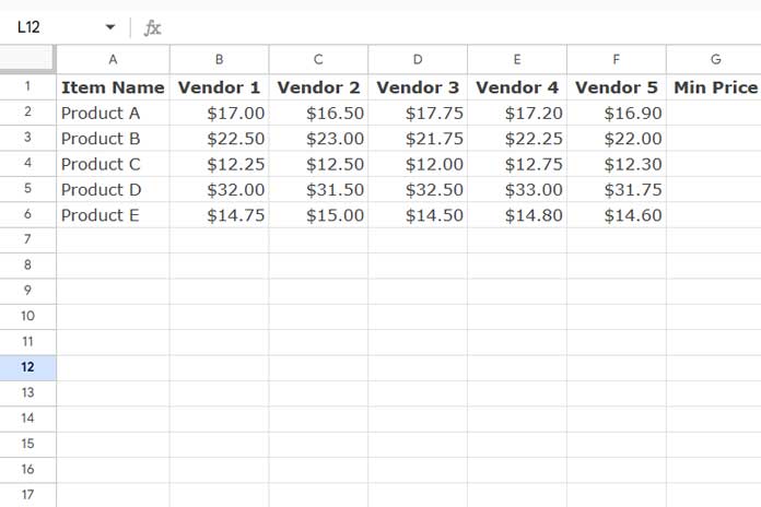
Finding the Lowest Price for Each Product
To find the lowest price for each product, you could start by using the MIN function in the first row to calculate the lowest price and then drag it down to apply it to other rows.
For example, enter the following MIN formula in cell G2 and drag it down to populate the lowest price for each product:
=MIN(B2:F2)However, we can also use array formulas to make this process more efficient, especially for large datasets or when you want results to update automatically.
In this tutorial, we’ll explore three formulas for finding row-wise minimum values across arrays:
- BYROW (using a LAMBDA function),
- DMIN (a database function), and
- QUERY.
Of these, BYROW and DMIN are the simplest to implement. I’ll include the QUERY method as well to demonstrate additional techniques.
Notes:
- While BYROW and QUERY can calculate row-wise minimums, both may face performance issues with very large datasets. DMIN tends to be more efficient and resilient with larger data.
- This guide follows a step-by-step approach to help you understand how each formula is developed. You can use the final formulas directly in the last parts of Methods 1, 2, and 3. The step-by-step breakdown is meant to enhance your understanding, not necessarily for direct implementation.
Method 1: MIN in Arrays for Expanded Results with BYROW
The numeric data is in the range B2:F. To find the minimum price for the first product in cell G2, you can use the following formula:
=MIN(B2:F2)Instead of dragging this formula down, you can convert it into a LAMBDA function and apply it to each row in the range B2:F using the BYROW function:
Step-by-Step
- Define the LAMBDA function:
LAMBDA(row, MIN(row))
In this custom function, we’ve defined the name “row” to represent each row in the range. - Use the BYROW function:
=BYROW(B2:F, LAMBDA(row, MIN(row)))
This formula will calculate the minimum for each row in the range B2:F. - Handle Empty Cells: If you want to avoid returning zero for empty cells, you can add a condition like this:
=ARRAYFORMULA(
   IF(
      A2:A="",,
      BYROW(B2:F, LAMBDA(row, MIN(row)))
   )
)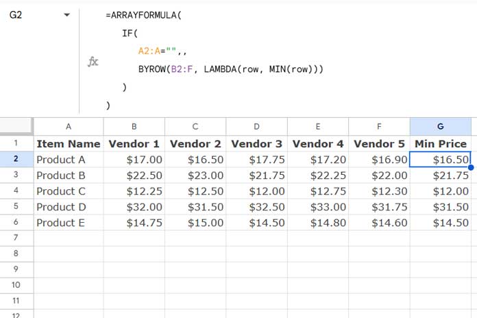
This is one of the easiest solutions to use the MIN function for expanded array results in Google Sheets.
Method 2: MIN in Arrays for Expanded Results with DMIN
While the DMIN function typically returns the minimum value of each column in structured data, we can use it to find the row-wise minimum by transposing the data.
Step-by-Step
- Transpose the Range: Use the following formula to transpose the numeric range:
=TRANSPOSE(B2:F6) - Add a Header Row: DMIN requires a header row for structured data. You can add a header using:
=VSTACK(TRANSPOSE(B2:B6), TRANSPOSE(B2:F6)) - Using DMIN: The syntax for DMIN is:
DMIN(database, field, criteria)
Here, the database is the VSTACK and TRANSPOSE combination.
The field should include all columns in the transposed data. To do this, use:SEQUENCE(ROWS(B2:B6)) - Set Criteria: Since we don’t want to filter the data using any criteria, you can represent it with two empty vertical cells:
{IF(,,); IF(,,)} - Final DMIN Formula: Enter the following as an array formula in cell G2:
=ArrayFormula(
   DMIN(
      VSTACK(TRANSPOSE(B2:B6), TRANSPOSE(B2:F6)),
      SEQUENCE(ROWS(B2:B6)),
      {IF(,,); IF(,,)}
   )
)
If you open the ranges, you may see zeros in empty rows. To handle this, you can use an IF logical test as shown below:
=ArrayFormula(
   IF(A2:A="",,
      DMIN(
         VSTACK(TRANSPOSE(B2:B), TRANSPOSE(B2:F)),
         SEQUENCE(ROWS(B2:B)),
         {IF(,,); IF(,,)}
      )
   )
)
Method 3: MIN in Arrays in Google Sheets Using QUERY
Similar to DMIN, the QUERY function can be used to return the minimum value in each column. We can transpose the range and return the minimum values, then transpose the result to obtain the row-wise minimum.
Step-by-Step
- Basic QUERY Formula:
=TRANSPOSE(QUERY(TRANSPOSE(B2:F6), "SELECT MIN(Col1), MIN(Col2), MIN(Col3), MIN(Col4), MIN(Col5)"))
This will return the result in two columns, where the first column contains the label “min”. - Using INDEX: To extract the second column, use:
=INDEX(TRANSPOSE(QUERY(TRANSPOSE(B2:F6), "SELECT MIN(Col1), MIN(Col2), MIN(Col3), MIN(Col4), MIN(Col5)")), 0, 2) - Automating the MIN Selection: The above formula isn’t dynamic since we manually specify the columns. To automate this, you can use:
=ArrayFormula(TEXTJOIN("),", TRUE, "MIN(Col"&SEQUENCE(COLUMNS(TRANSPOSE(B2:F6))))&")")
You can replace the manual"MIN(Col1), MIN(Col2), …"part of the QUERY string with this formula, eliminating the need for the ARRAYFORMULA function. - Final Dynamic QUERY Formula: The final formula will be:
=INDEX(TRANSPOSE(QUERY(TRANSPOSE(B2:F6), "SELECT "&TEXTJOIN("),", TRUE, "MIN(Col"&SEQUENCE(COLUMNS(TRANSPOSE(B2:F6))))&")")), 0, 2)
As a best practice, I suggest using closed ranges to prevent performance issues.
Conclusion
In this tutorial, we explored three methods for finding the row-wise minimum values in Google Sheets: using BYROW, DMIN, and QUERY. Each method has its strengths, and you can choose the one that best fits your data structure and performance needs.
I hope you learned some useful tips on how to utilize the MIN function effectively with arrays in Google Sheets!
Resources
- Filter Min or Max Value in Each Group in Google Sheets
- How to Highlight the Min Value in Each Group in Google Sheets
- Get Max Date in Each Row Using an Array Formula in Google Sheets
- How to Find Max Value in Each Row in Google Sheets
- Return First and Second Highest Values in Each Row in Google Sheets


