Find and Filter the Min or Max Value in Groups in Google Sheets

This tutorial explains how to find and filter the minimum or maximum value in each group in Google Sheets using a formula or the Filter command.

Use the formula when you want to extract the smallest or largest values for each group into a new range. Use the Filter command when you want to display only the relevant values within the source data.

Find the MIN Values in Groups (Formula Approach)

You might want to find the minimum value in groups with or without a date column. The formula varies depending on the scenario.

Example 1: Finding the Lowest Value in Each Group

Consider the following sample data (A1:B):

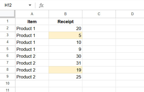
Sample data for filtering minimum or maximum values by group

To get the minimum value in each group, use the following QUERY formula:

=QUERY(A1:B, "select Col1, min(Col2) where Col1 is not null group by Col1")

This will return the minimum receipt quantity for each product:

Item	min Receipt
Product 1	5
Product 2	19

How the Formula Works:

A1:B -> The data range.
Col1 -> The grouping column (adjust it if your grouping column is different, e.g., Col4 for column 4).
Col2 -> The column from which to extract the lowest value.

Notes:

Column numbers are relative to the range, not the sheet.
To modify the labels in the result, use the LABEL clause in QUERY.

Example 2: Finding the Lowest Value in Each Group by Date

In certain cases, you may want to find the minimum value in each group based on date, such as tracking the lowest sales per product per day.

Here’s a sample dataset (A1:C):

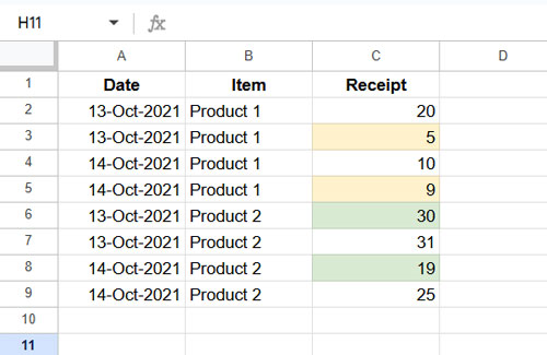
Sample data for filtering minimum or maximum values by group and date

To find the lowest value per group and date, use:

=QUERY(A1:C, "select Col2, Col1, min(Col3) where Col1 is not null group by Col2, Col1")

Result:

Item	Date	min Receipt
Product 1	13-Oct-2021	5
Product 1	14-Oct-2021	9
Product 2	13-Oct-2021	30
Product 2	14-Oct-2021	19

How the Formula Works:

A1:C -> The data range.
Col2 -> The first column to group by (Item/Category).
Col1 -> The date column.

Find the MAX Values in Groups (Formula Approach)

To find the maximum values in each group, replace the min function with max in the formulas.

Example 1: Finding the Largest Value in Each Group

=QUERY(A1:B, "select Col1, max(Col2) where Col1 is not null group by Col1")

Item	max Receipt
Product 1	20
Product 2	31

Example 2: Finding the Largest Value in Each Group by Date

=QUERY(A1:C, "select Col2, Col1, max(Col3) where Col1 is not null group by Col2, Col1")

Item	Date	max Receipt
Product 1	13-Oct-2021	20
Product 1	14-Oct-2021	10
Product 2	13-Oct-2021	31
Product 2	14-Oct-2021	25

Find the MIN or MAX Values Using the Filter Command

Filtering the source data directly has two advantages:

You can see and edit the results in the original range.
You avoid creating additional ranges, keeping your sheet clean.

To filter the min or max values by group, apply the filter function to the numeric column.

Example 1: Filtering the Smallest Value in Each Group

We will use the same two-column dataset, where Item is in column A and Receipt in column B.

Steps:

Select B1:B.
Click Data > Create a Filter.
Click the filter drop-down in B1.
Select Filter by condition > Custom formula is.
Enter the formula:
=B2=MINIFS($B$2:B, $A$2:$A, A2)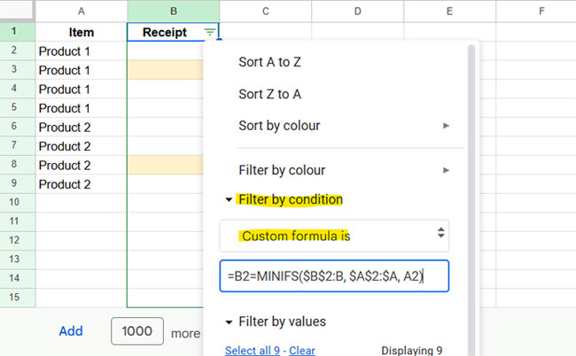
Click OK.

This filters the smallest values in each group.

How the Formula Works:

MINIFS($B$2:B, $A$2:$A, A2)

MINIFS finds the smallest value in B2:B, where A2:A matches the item in A2.
This applies to each row as A2 updates to A3, A4, and so on within the filter range.

=B2 checks whether each row’s value matches the minimum value in its group. If it does, the row is included in the filter.

Example 2: Filtering the Largest Value in Each Group

To filter the maximum value instead, use:

=B2=MAXIFS($B$2:B, $A$2:$A, A2)

Example 3: Filtering the Smallest Value in Each Group by Date

If dates are in column A, items in column B, and receipt quantities in column C, use:

Select C1:C.
Click Data > Create Filter.
Click the filter drop-down in C1.
Select Filter by condition > Custom formula is.
Enter:
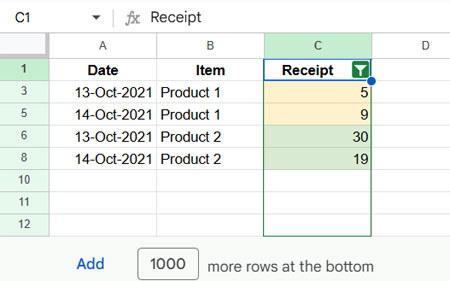
=C2=MINIFS($C$2:C, $A$2:$A, A2, $B$2:$B, B2)
Click OK.

This filters the smallest values in each group by date and category.

Filter menu to filter the minimum value by category and date

How the Formula Works:

MINIFS($C$2:C, $A$2:$A, A2, $B$2:$B, B2) finds the minimum value in C2:C where A2:A = A2 and B2:B = B2.
If C2 matches this minimum, the row is shown in the filter.

This applies to each row in the range.

Example 4: Filtering the Largest Value in Each Group by Date

Simply replace MINIFS with MAXIFS:

=C2=MAXIFS($C$2:C, $A$2:$A, A2, $B$2:$B, B2)

FAQs

Does the formula update when new data is added?

Yes, since we use open-ended ranges, the formula captures new values dynamically.

Does the filter menu refresh automatically when new values are added?

No, you must click the filter drop-down and select OK to refresh the filtered data.