How to Find the Highest N Values in Each Group in Google Sheets

You can interpret the highest N values in each group in two main ways:

Highest N Values + Duplicates of the Nth Highest
Unique Top N + All of Their Duplicates

The formula varies depending on your specific needs. Please refer to the table below before proceeding to the formulas:

Formula Selection Criteria

Values	Top 3 + All Duplicates of Nth	Top 3 (Distinct Values + All Occurrences)
30	✅	✅
20	✅	✅
20	✅	☑️
20	☑️	☑️
11		✅
11		☑️
10

Find the Highest N Values in Each Group + Duplicates of Nth

To find the highest N values and include duplicates of the Nth value, if any, within each group in Google Sheets, use the following formula:

=FILTER(A2:C, B2:B<>"", COUNTIFS(B2:B, B2:B, C2:C, ">"&C2:C)+1<=10)

Formula Components:

A2:C: The data range to filter
B2:B: The category/group column
C2:C: The score/qty/amount column
10: The number of top values to retrieve

Find the Top N Values in Each Group + Their Duplicates

To retrieve the top N unique values and their duplicates, if any, within each group, use this formula:

=ArrayFormula(LET(
   data, A2:C, category, B2:B, score, C2:C, n, 10, 
   unq, UNIQUE(HSTACK(category, score)), 
   colA, CHOOSECOLS(unq, 1), colB, CHOOSECOLS(unq, 2), 
   rnk, COUNTIFS(colA, colA, colB, ">"&colB)+1, 
   keys, IF(rnk<=n, colA&colB,), 
   FILTER(data, category<>"", XMATCH(category&score, keys))
))

Formula Components:

A2:C: The data range to filter
B2:B: The category/group column
C2:C: The score/qty/amount column
10: The number of top values to retrieve

Example 1: Finding the Highest N Values + Duplicates of Nth in Each Group

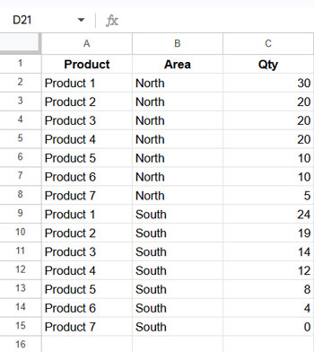
Consider the following dataset containing Product Names, Area, and Sales Volume:

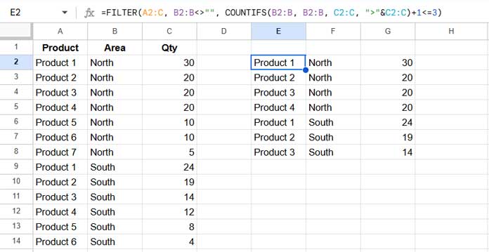
Sample Data Showing Sales Volume by Region

Now, if you want to identify the top 3 selling items in each region based on sales volume, use this formula:

=FILTER(A2:C, B2:B<>"", COUNTIFS(B2:B, B2:B, C2:C, ">"&C2:C)+1<=3)

Expected Output:

Finding the Top N Values and Duplicates of the Nth Highest in Each Group

Formula Explanation:

COUNTIFS(B2:B, B2:B, C2:C, ">"&C2:C) + 1: Calculates group-wise ranking, where the group is the Area column and the rank is based on Sales Volume.
B2:B<>"" : Ensures that only non-empty category rows are considered.
The FILTER function then extracts only the top 3 values per group.

This is one way to find the highest N values in each group on Google Sheets. Now, let’s look at another example.

Example 2: Finding Unique Highest N Values + Their Duplicates in Each Group

Dataset Example (A1:C)

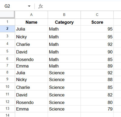
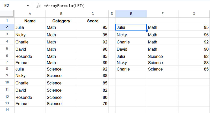
To find the highest N values in each group (e.g., the top 3 scores per subject), enter this formula:

=ArrayFormula(LET(
   data, A2:C, category, B2:B, score, C2:C, n, 3, 
   unq, UNIQUE(HSTACK(category, score)), 
   colA, CHOOSECOLS(unq, 1), colB, CHOOSECOLS(unq, 2), 
   rnk, COUNTIFS(colA, colA, colB, ">"&colB)+1, 
   keys, IF(rnk<=n, colA&colB,), 
   FILTER(data, category<>"", XMATCH(category&score, keys))
))

Expected Output:

Formula to Filter the Top 3 Unique Values and Their Duplicates in Each Group in Google Sheets

This formula efficiently handles ties when filtering the top N values in each group.

Formula Logic Breakdown:

UNIQUE(HSTACK(category, score)): Extracts unique category-score combinations.
COUNTIFS(colA, colA, colB, ">" & colB) + 1: Ranks scores within each category.
IF(rnk <= n, colA & colB, ""): Identifies the top N values in each group.
FILTER(data, category <> "", XMATCH(category & score, keys)): Filters and returns the top N values in each group.

This method ensures that only the highest-ranked values per category are displayed efficiently.

Common Questions

Do these formulas work on unsorted data?

✅ Yes, they work on both sorted and unsorted data. Sorting is not required.

Are these formulas resource-intensive?

✅ No, they are optimized for performance. However, for large datasets, performance may be impacted due to ampersand (&) limitations when combining multiple columns.

Additional Resources

31 COMMENTS

Taylor Wilson June 9, 2023 At 3:13 am

Hello,

I was wondering, if you knew how to accomplish this with two columns identifying the grouping.

I have ten records for a person on a given date/time and need the top 5 values from that day. Also I need another top 5 for a different day for the same person.

I have tried joining the Name and Date column to make a unique value but needed to split after. Wondering, if there is a simpler way.

Name, Date, Score
A, Jan 1, 20
A, Jan1, 40
A, Feb 1, 34
A, Feb 1, 33
B, Jan 1, 20
B, Jan 1, 30

Becomes…

Name, Date, Score
A, Jan 1, 40
A, Feb 1, 34
B, Jan 1, 30

It is expanded out to 10 records each day per person.

- Prashanth June 9, 2023 At 9:56 am
  
  Hi, Taylor Wilson,
  
  First and foremost, I’ve updated my formula in the post to enhance its performance using LET. Please check that.
  
  Then regarding your question, we can do it as follows.
  
  But before that, I could understand you have a Name and Date column.
  
  If the Date column contains timestamps, you must remove the time element. So that grouping will work.
  
  Range: A1:C
  
  Where; A1, B1, and C1 contain the field labels Name, Date, and Score, respectively.
  
  Formula:
  
  =LET(sorted,SORT(A2:C,1,true,2,true,3,false), ARRAYFORMULA(QUERY(HSTACK(sorted,IFERROR(ROW(A2:A)- MATCH(CHOOSECOLS(sorted,1)&CHOOSECOLS(sorted,2), CHOOSECOLS(sorted,1)&CHOOSECOLS(sorted,2),0))), "Select Col1,Col2,Col3 where Col4<6")))
  
  - Taylor Wilson June 30, 2023 At 8:27 pm
    
    Hello Prashanth,
    
    Ah, I did not see your update.
    
    Amazing, this is spot on.
    
    Thank you so much!
    
Rach March 18, 2022 At 7:12 am

Hi Prashanth,

I just found this post, and thank you for this tutorial, I found it very helpful as I needed it, and I have a question, though.

If I have two or more groups, let’s say four columns; Level 0, Level 1, Level 2 groups and scores, and I want to sort it by top five and bottom five, from every Level 2 by each Level 0.

How to make it happen? Thanks.

- Prashanth March 18, 2022 At 11:02 am
  
  Hi, Rach,
  
  It seems doable!
  
  I highly recommend you to share a sample/mockup sheet with me below. Include your hand entered (expected) result.
  
  I will try to solve it ASAP.
  
  - Rach March 18, 2022 At 1:24 pm
    
    Hi, Thank you. Below is the sample sheet.
    
    — link (URL) removed by the Admin —
    
    - Prashanth March 20, 2022 At 10:29 am
      
      Hi, Rach,
      
      I have added the required formulas to your sheet.
      
      Thanks for sharing an easy-to-read sample sheet.
      
Desmond Lee January 13, 2022 At 7:26 pm

Hi, There,

Column M contains mixed Text and Numbers like this;

2160
2732
M293
2739
NP018
M149

Where can’t I replace M2:M with TO_TEXT(M2:M)?

- Prashanth January 14, 2022 At 10:10 am
  
  Hi, Desmond Lee,
  
  The best way is to select M2:M and apply Format > Number > Plain text.
  
  If you do not want to format it like that, I have a new formula that works well with all data types. Here it is.
  
  =filter(sort(A2:B,1,1,2,0),countifs(sort(A2:A,1,1,2,0),sort(A2:A,1,1,2,0), row(A2:A),"<="&row(A2:A))<3)
  
Caleb November 25, 2020 At 1:12 am

Hello,

Thanks for the formula and it works exactly like you said it would. However, I am limiting my results to where I will need at least 5 occurrences to get a proper score.

With your formula, it will show everyone even those that only have one result which is exactly how it is programmed. Is there a way to limit the data to show those that have at least 5 results? Sorry if I didn’t explain it very well and I can try to clarify more if needed.

Caleb

- Prashanth November 26, 2020 At 12:07 pm
  
  Hi, Celeb,
  
  We can achieve this without much effort.
  
  Assume my data is in Sheet1!A2:B (as per my example above). If so, in another blank sheet (let’s call it Sheet2) in the same file, in cell A2, insert the below Filter.
  
  =filter(Sheet1!A2:B,countif(Sheet1!A2:A,Sheet1!A2:A)>=5)
  
  Use the formula given in my tutorial with this data in Sheet2, not with the one in Sheet1.
  
David September 4, 2020 At 7:42 am

Thank you very much for your post. I found it very helpful! I do have a question though.

In my case, I need to get the highest three dates for a trailer number that is NOT greater than today’s date. Any suggestions on how to accomplish this using your methodology? Thank you for your help!

- Prashanth September 4, 2020 At 1:25 pm
  
  Hi, David,
  
  You want a formula that returns the highest n dates that are less than or equal to today’s date. Also, it should be based on a criterion, i.e. Trailer number.
  
  Eg.
  
  A2:A contains dates.
  B2:B contains trailer numbers (for example “XY 10001”)
  (titles in A1:B1)
  
  Here in this case, in cell C2 use this formula.
  
  =sortn(filter(A2:A,B2:B="XY 10001",A2:A<=today()),3,0,1,0)
  
  I know the SORTN parameters, i.e. 3,0,1,0, maybe a little bit confusing.
  
  3 = number of values to return ('n')
  0 = Show at most the first 'n' rows in the sorted range.
  1 = sort column number (date column).
  0 = sort in descending order.
  
  This formula may return the same dates if there are duplicates. So here is a more refined one to extract the top 3 dates without duplicates based on a condition.
  
  =sortn(filter(A2:A,B2:B="XY 10001",A2:A<=today()),3,2,1,0)
  
  If you face issues using the above formulas, feel free to share the URL of a mockup sheet.
  
Aaron August 5, 2020 At 6:55 pm

Hi, I can’t seem to get my formula to work correctly. It says there is an error with the last part of the formula
“Array Formula only takes 1 Argument, but this is argument 2”

On the transactions sheets, the rows are A(Date), B (Category), C (Description), D (Amount), E (Account).

- Prashanth August 7, 2020 At 2:27 pm
  
  Hi, Aaron,
  
  If you share a mockup sheet, I would be happy to assist you.
  
Ron June 28, 2020 At 4:34 pm

Hi Prashanth,

Thanks for all your help with this. I guess now I will learn how to get rid of dashes when importdata via the =importhtml command:>) I will let you know if I find out.

PS: I tried using rank out of curiosity, voila it works, it correctly highlights the top 10 in each column, and does not highlight the dashes. Formula: =RANK(C3,C$3:C$121)<=10. See the example in sheet 3.

Regards,

Ron.

- Prashanth June 29, 2020 At 9:01 am
  
  Hi, Ron,
  
  Thanks for sharing your formula. It works well!
  
  Cheers!
  
Ron June 28, 2020 At 6:49 am

Hi Prashanth,

Can you please explain how this formula works, I see that it selects the first cell in the range, does the = after C3 mean that it looks in the whole range to look for dashes, but then I do not understand how the dashes are removed, as I cannot see this in the function?

- Prashanth June 28, 2020 At 7:43 am
  
  Hi, Ron,
  
  You are absolutely right. It’s called the relative reference. Read more about here – Relative Reference in Conditional Formatting in Google Sheets.
  
  To remove the cell color, I have used white as the cell fill color in that rule. You can even hide the hyphen by changing the font color to white in the same formula rule.
  
  So no need to specify the same in the formula.
  
Ron June 26, 2020 At 4:40 pm

Hi Prashanth,

That function works, however as some fields have dashes, it highlights them as well, thereby creating additional highlighted fields. How do you exclude dashes in the function for the given range?

Here is the link to the file: removed_by_admin

- Prashanth June 27, 2020 At 2:04 pm
  
  Hi, Ron,
  
  Added a new rule to “Sheet2” in your file to remove highlighting the rows containing the hyphen character. It’s below.
  
  =C3="-"
  
  The above should be the first rule in the order.
  
Ron June 26, 2020 At 8:37 am

Hi Prashanth,

Thanks for the code it works a treat. If I want to confirm the top 10 in each column I just use Rank <=10, instead of max, correct.

- Prashanth June 26, 2020 At 9:29 am
  
  Hi, Ron,
  
  I think it won’t work. Try this formula.
  
  =B$3:B$15>=large(arrayformula(n(B$3:B$15)),10)
  
  This range is as per my previous answer.
  
Ron June 22, 2020 At 9:44 am

Hi Prashanth,

I have a query about dynamically highlighting or identifying the highest value in each of five different columns (eg say 1 Mth, 3 Mths, 1 Yr, 3 Yrs & 5 Yrs.

What I would like to happen is when I open the Google worksheet it would automatically highlight the highest value in each of the five-column ranges.

Is it possible to do this under Conditional Formatting or does it have to be done via a Query? Please advise how I could achieve this.

- Prashanth June 22, 2020 At 3:04 pm
  
  Hi, Ron,
  
  Yes! It’s possible using the “Format > Conditional formatting > Format rules > Custom formula is” in Google Sheets.
  
  Assume the columns (1 Mth, 3 Mths, 1 Yr, 3 Yrs & 5 Yrs) to highlight are B3:F (5 columns).
  
  With a single conditional format formula in Google Sheets, we can highlight the max values in each column.
  
  In conditional formatting enter B3:F in “Apply to range” field.
  
  Under “Custom Formula is” field (click the drop-down under “Format rules”) insert the following formula.
  
  =B$3:B=max(B$3:B)
  
  For the range B3:F100, the formula to use would be as below.
  
  =B$3:B$100=max(B$3:B$100)
  
  I hope this helps?
  
Punchcruff August 24, 2019 At 3:13 am

I can’t seem to get this to work for some reason. I even tried removing the “row(A2:A)-” like the person above suggested, but that resulted in an error stating “Function ARRAY_ROW parameter 2 has mismatched row size. Expected: 999. Actual: 995.”

For reference, the data I’m working with is 3 columns: Name, Team, Score. My goal is to find the highest score from each team and to display the team, score, and corresponding name.

I’ve come very close a number of times, but for some reason, it’s failing to actually display the highest record–it seems to be picking one from the middle.

Also, you explain that this formula adds in an extra column. While I’ve been operating with trust in what you’ve said, I’ve so far failed to identify wherein the logic that is dictated. Would you mind elaborating?

The formula I’ve ended up with is:

=ArrayFormula(QUERY({SORT(B2:D,2,true,3,false),IFERROR(row(B2:B)-match(query(SORT(B2:D,2,true,3,false),"Select Col3"),query(SORT(B2:D,2,true,3,false),"Select Col3"),0))},"Select Col1, Col2, Col3 where Col4<2"))

Column B is the name, Column C the team, and Column D the score.

Thank you in advance for any insight you can provide!

- Prashanth August 24, 2019 At 3:35 pm
  
  Hi, Punchcruff,
  
  You were very close with your above attempt.
  
  I assume, your data range is B2:D. In that, you want to sort the Team column (column C). You have correctly made changes in the SORT formulas.
  
  But in the inside Query formulas, instead of column 2, the sort column, you have put 3. That’s the only issue.
  
  Here is the correct formula.
  
  =ArrayFormula(QUERY({SORT(B2:D,2,true,3,false),IFERROR(row(B2:B)-match(query(SORT(B2:D,2,true,3,false),"Select Col2"),query(SORT(B2:D,2,true,3,false),"Select Col2"),0))},"Select Col1,Col2,Col3 where Col4<2"))
  
  Regarding the extra column, it is the grouped numbers. To see that use this formula.
  
  =ArrayFormula(QUERY({SORT(B2:D,2,true,3,false),IFERROR(row(B2:B)-match(query(SORT(B2:D,2,true,3,false),"Select Col2"),query(SORT(B2:D,2,true,3,false),"Select Col2"),0))},"Select * where Col4<2"))
  
  The above formula is useful to return the highest 'N' values. In your case, you want to find the highest 1 score from each team, not the highest 'N'. It can simply achieve with the below SORTN formula.
  
  =sortn(sort(B2:D,3,0,2,1),9^9,2,2,0)
  
  See the below two guides to learn the function used here.
  
  1. How to Use SORTN Function in Google Sheets to Extract Sorted N Rows.
  2. SORTN Tie Modes in Google Sheets – The Four Tiebreakers.
  
  Best,
  
  - Punchcruff August 26, 2019 At 7:32 pm
    
    My apologies about the column–I knew that wasn’t correct, but had been trying whatever I could, and mistakenly copied the formula without correcting it. However, the formula still returns a value from the middle of each team, not the highest.
    
    Regardless, though, I’ll be trying out the SORTN function, and seeing if that can provide results with more ease.
    
    Thank you for your help!
    
  - Punchcruff August 26, 2019 At 8:03 pm
    
    The SORTN formula you wrote worked for me! Thanks again!
    
    - Prashanth August 27, 2019 At 8:20 am
      
      Thanks for the feedback!
      
Kostya July 30, 2019 At 2:46 am

Thank you for this tutorial, works like a charm for me.

The only change that I needed to do, is to remove “row(A2:A)-” from the formula