Combining (appending) data from multiple sheets horizontally in Google Sheets may not be a frequently required task, as it may not always contribute to data manipulation efficiency.

The preferred approach is often to combine multiple sheets vertically. However, there are scenarios where combining sheets horizontally becomes necessary.

For instance, imagine a Google Sheets file with twelve sheets, each representing data for the months Jan to Dec. Column A in all sheets contains the names of employees in the same order, while Column B represents their monthly gross salary, which varies on each sheet.

In such cases, the need to combine data horizontally across the 12 sheets into a master sheet may arise. This facilitates streamlined data manipulation and provides a comprehensive view of all data in one location.

The most straightforward method to append multiple sheets horizontally is by specifying the ranges within the HSTACK function. If you prefer a more dynamic approach to combining multiple sheets horizontally, you can utilize a modern technique that involves the REDUCE function.

The Fastest Way to Append Data Horizontally

We can’t proceed without showcasing our sample data because ‘everything’ revolves around it.

There are five sheets in a Google Sheets file named Jan, Feb, Mar, Apr, and Merged.

We will combine the data in cell range A1:B in the first four sheets horizontally into the fifth sheet.

The fifth sheet is currently blank. We will horizontally combine data from the above four sheets into that sheet.

The quickest way to append data horizontally is to use the HSTACK function.

Syntax: HSTACK(range1, [range2, …])

Insert this formula into cell A1 on the “Merged” (fifth) sheet.

=IFERROR(HSTACK(Jan!A1:B, Feb!A1:B, Mar!A1:B, Apr!A1:B))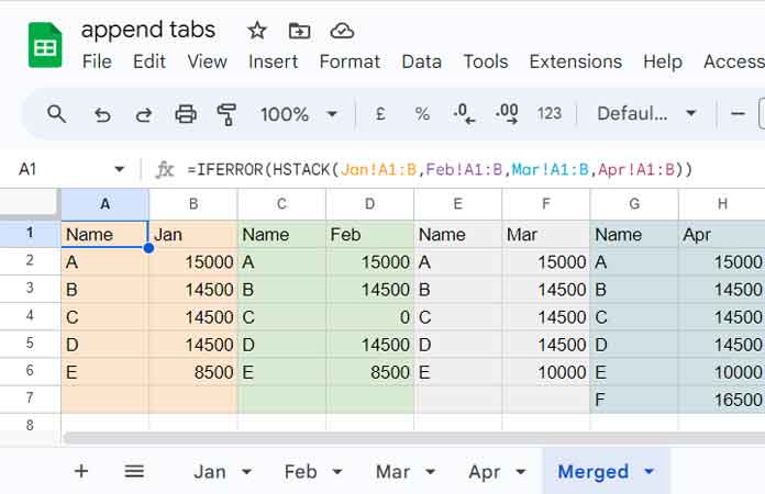

You can use open ranges (e.g., Jan!A1:B) or closed ranges (e.g., Jan!A1:B6) in the formula.

If you want to import only part of the data from one sheet and merge it with the total data from other sheets, don’t worry! You can combine multiple sheets horizontally with an unequal number of rows.

=IFERROR(HSTACK(Jan!A1:B5, Feb!A1:B5, Mar!A1:B100, Apr!A1:B100))

The above Google Sheets formula will return five rows from the first two sheets and a hundred rows from the other two sheets. We have utilized the IFERROR function to mitigate errors that may arise from appending tables with unequal rows.

You can arrange the sheets in the order you want in the formula.

Combine Multiple Sheets Horizontally by Referring to Sheet Names in a Range

In August 2022, Google Sheets introduced a powerful bundle of functions that has since proven to be transformative and life-changing.

One notable function within this bundle is REDUCE, serving as a LAMBDA helper function. Its introduction has significantly altered the way we interact with Google Sheets.

The use of LAMBDA is particularly crucial for referencing a list of sheet names (as opposed to just one sheet) within formulas.

Here’s a guide on how to utilize REDUCE to dynamically combine data horizontally from multiple sheets based on a list of sheet names within a specified range.

Dynamically Combine Multiple Sheets Horizontally Using the REDUCE Function

We can utilize the REDUCE function to dynamically combine multiple sheets horizontally.

What’s more, you can use it to combine data from the first sheet to the last sheet or vice versa. We will begin with the first to last.

Assuming the fifth sheet is empty, if you have the aforementioned HSTACK formula in it, please remove it.

Enter the sheet names in cells A1 to A4 in this sheet (there are four sheets in the workbook from which we want to import data and append them horizontally).

Next, insert the following REDUCE formula in cell B1.

=REDUCE(
   TOROW(, 1), 
   TOCOL(A1:A, 1), 
   LAMBDA(a, v, IFERROR(HSTACK(a, INDIRECT(v&"!A1:B10"))))
  )

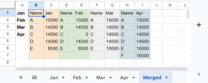
It appends data from the range A1:B10 using the sheet names entered in A1:A.

This implies that you should modify A1:A and A1:B10 in the formula to adapt it to your list containing sheet names and the data range you want to combine.

How Does the REDUCE Combine Data Horizontally in Google Sheets?

Let’s delve into the syntax of the REDUCE function:

Syntax: REDUCE(initial_value, array_or_range, lambda)

• initial_value: TOROW(, 1)

The TOROW function will return an empty cell if specified as TOROW(, 0). By changing 0 to 1, it eliminates that empty cell. Thus, it serves the initial_value requirement for REDUCE. It essentially returns nothing.

• array_or_range: TOCOL(A1:A, 1)

It returns the list of sheet names, removing empty cells.

In the formula (within lambda):

• a: name of the accumulator.
• v: each value (sheet name) from array_or_range.

The REDUCE function iterates over each sheet name in the array_or_range, using the function INDIRECT(v&"!A1:B10"). In each iteration, the v represents Jan (Sheet1,) Feb (Sheet2,) Mar (Sheet3,) and Apr (Sheet4.)

The result at each step is stored in the accumulator, which is then horizontally stacked using HSTACK as HSTACK(a, …). This outlines the REDUCE logic behind dynamically combining multiple sheets.

Horizontal Merging from Last Sheet to First Sheet

Do you want to append data from the last sheet to the first sheet?

In other words, merge data from sheets horizontally in the order Apr, Mar, Feb, and Jan, rather than Jan, Feb, Mar, and Apr.

It’s straightforward with the REDUCE formula above. Instead of using HSTACK(a, v), utilize HSTACK(v, a) as follows.

=REDUCE(
   TOROW(, 1), 
   TOCOL(A1:A, 1), 
   LAMBDA(a, v, IFERROR(HSTACK(INDIRECT(v&"!A1:B10"), a)))
  )

Removing Repeated First Column

One of the issues you may face while combining data horizontally is the repetition of one of the columns, possibly the first one contains a common description.

In my example, how do we remove the multiple occurrences of the “Name” column?

The solution is quite simple.

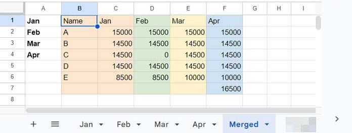
Do not include the first column in the REDUCE formula. I mean, replace v&"!A1:B10" with v&"!B1:B10".

Then use the formula inside an HSTACK and here it is.

=HSTACK(Jan!A1:A10, 
   REDUCE(
      TOROW(, 1), 
      TOCOL(A1:A, 1), 
      LAMBDA(a, v, IFERROR(HSTACK(a, INDIRECT(v&"!B1:B10"))))
   )
)

Another option is to encapsulate my original formula within CHOOSECOLS or QUERY to extract the specific columns we need from the appended sheets’ data.

Resources

Above, we have seen how to combine data horizontally using a simple HSTACK or using REDUCE, a dynamic approach. Here are some resources that handle similar topics.

• Consolidate Data from Multiple Sheets Using a Formula in Google Sheets
• Consolidate Only the Last Row in Multiple Sheets in Google Sheets
• How to Combine Multiple Sheets in Importrange and Control Via Drop-Down
• SUMIF Across Multiple Sheets in Google Sheets
• Vlookup Across Multiple Sheets in Google Sheets
• How to Include Future Sheets in Formulas in Google Sheets